What you will learn
This notebook will teach you to:- Create a WherobotsDB context
- Load raster and vector geospatial data from AWS S3 buckets into DataFrames
- Streamline geospatial workflows using temporary views
- Filter, query, and manipulate geospatial data using Spatial SQL
- Calculate zonal statistics — like mean temperature over spatial geometries — using
RS_ZonalStats - Visualize data and explore insights using SedonaKepler
Set up your Sedona context
ASedonaContext connects your code to the Wherobots Cloud compute environment where your queries can run fast and efficiently.
First, you set up the config for your compute environment, then use that configuration to launch the sedona context. We’ll use the default configuration in this notebook, but you can learn about configuring the context in our documentation.
Using vector data
Wherobots is a cloud-native tool and works best with data in cloud storage. In this notebook, we will an example dataset, but when you want to work with your own data, you have two options:- Load your data into Wherobots Cloud managed storage, our managed solution
- Connect to AWS S3 buckets and integrate with existing data workflows
Vector data is spatial data that includes geometry like points, lines, and shapes.We will use the following code snippet to load a GeoParquet file from S3 into a Sedona DataFrame.
GeoParquet is an open, efficient format for storing geospatial data, perfect for large-scale geospatial workflows. (Docs: Loading GeoParquet)
Using raster data
Wherobots lets you write queries that combine vector and raster data.Raster data is spatial data that has one or more values stored in a grid. Satellite photography is one kind of raster data, where each grid location has a red, green, and blue value that are combined to create the color of the corresponding pixel. Two common raster formats are GeoTIFF and COG (Cloud Optimized GeoTIFF).We will load a GeoTIFF raster file of the area near Central Park in New York City. This TIFF is not an image file, but a Digital Elevation Model (DEM), where each value in the grid represents the elevation of that point. This file uses a one-foot resolution, so each value represents the elevation of 1 square foot (0.093 sqare meters) of the park. (Docs: Raster Loaders)
rastcontains a tile that is one part of the overall rasterxandyare the coordinates of the tile within the rasternameis the original file name (CentralPark.tif) for all rows
Spatial SQL prefixes many function calls with eitherRS_(for “raster”) or, as you’ll see below,ST_(for “spatial-temporal”).
Writing SQL using temporary views
The line of code below callscreateOrReplaceTempView() to register our DataFrame as a temporary SQL view in Apache Spark. Temporary views allow you to interact with the DataFrame using SQL queries. For example, after creating the temporary view, you can run the following query to analyze the elevation data:
Querying with vector and raster data together
A simple way to combine vector and raster data is to look up a raster value at a specific point. For example, if we wanted to get the elevation of Strawberry Fields in Central Park, we can write that in Spatial SQL.RS_Value(rast, ST_Point(...))retrieves the value (in this case, elevation) from the raster value at the specified point (the longitude and latitude of Strawberry Fields).AS elevation_in_feetnames the output column.FROM elevationuses the temporary view we created.WHERE RS_Intersectskeeps only the raster tile that includes our point of interest.
WHERE clause, this query would return 1,872 rows, one for each tile in the raster. One row would have a numeric value for elevation_in_feet and the other 1,871 values would be NULL because their rast tile does not contain the point in question.
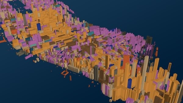
Visualizing data on a map using SedonaKepler
Kepler.gl is an open source map visualization tool that integrated into Wherobots asSedonaKepler. Here, we will use Kepler to show the buildings vector data we loaded previously. You can customize your map with Kepler.gl configuration settings that might start something like this:
config.json file that we will load into a dictionary called map_config, and then pass that dictionary as a parameter.
Analyzing building elevations across Central Park
Combining all the concepts we’ve covered so far, we will now calculate a zonal statistic, the average elevation for the buildings inside Central Park.A zonal statistic is an aggregate of values (like a sum, average, count, or maximum) across a geographic region.First, we will get set up for the query.
2263. This number is an entry in the EPSG catalog that refers to the NAD83 / New York Long Island coordinate reference system. However, our buildings vector data uses epsg:4326, the WGS84 Geographic Coordinate System, which uses latitude and longitude in decimal degrees. In order for us to do our query that joins across these two data sets, we will use ST_Transform to map buildings from the latter to the former.
Let’s get to the actual analysis.
elevationis raster data loaded from our Digital Elevation Model (DEM) GeoTIFF.buildingsis vector data of all the buildings in New York City, including their geometry (geom) and addresses (PROP_ADDR).
RS_ZonalStats computes the mean elevation for each building’s geometry based on the DEM:
- Raster input:
elevation.rastElevation raster values - Vector geometry: The shapes of the buildings
- Band:
1tells Wherobots to use the first band (value) of the raster (in this case, the elevation). - Statistic:
meancalculates the average within the vector geometry. - Ignore NoData:
trueensures invalid or missing data in the raster is excluded.
RS_Intersects ensures only raster values that intersect the buildings’ geometry are used.
Filtering results: Remove buildings with non-positive elevation values using WHERE elevation > 0.
Aggregation: Elevations are grouped by building address (PROP_ADDR) and geometry to compute the average elevation for each building.
Output: The resulting DataFrame, buildings_elevation, contains:
name: property address of the buildinggeom: building geometryelevation: average elevation of the building footprint (in feet)
Next steps
Congratulations on completing this notebook! You’ve learned how to:- Combine raster and vector data to derive meaningful insights about urban infrastructure. For example, it can be used for:
- Identifying buildings at risk of flooding based on elevation.
- Urban planning and construction in areas with varying terrain.
- Environmental impact studies within Central Park and surrounding areas.
- Perform zonal statistics to derive meaningful insights from elevation and temperature datasets.
- Use Apache Sedona SQL to manipulate and query spatial data efficiently.
🛠️ Experiment with Different Data Sources
- Use additional raster datasets, such as vegetation indices or precipitation maps, to enhance your analysis.
- Incorporate demographic or socioeconomic vector datasets to explore spatial relationships.
- Try quantifying health of crops and forests using NDVI analysis
- Use Overture Maps data hosted and managed by Wherobots
🔍 Try Advanced Apache Sedona Features
- Explore Sedona’s spatial join capabilities to analyze relationships between multiple vector datasets.
- Use Sedona’s advanced functions, like
ST_BufferorST_Within, for proximity and containment analysis. - Check out our full function reference for Apache Sedona here.