The following content is a read-only preview of an executable Jupyter notebook.To run this notebook interactively:
  1. Go to Wherobots Cloud.
  2. Start a runtime.
  3. Open the notebook.
  4. In the Jupyter Launcher:
    1. Click File > Open Path.
    2. Paste the following path to access this notebook: examples/Getting_Started/Part_2_Reading_Spatial_Files.ipynb
    3. Click Enter.
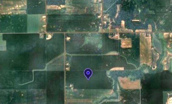
Welcome to this notebook on loading raster and vector data. In this notebook, you will learn how to load a variety of formats from cloud storage and Wherobots managed storage. Map pointer on satellite image of crop fields Vector data represents discrete features like points, lines, and polygons. Common formats include:
  • GeoParquet: Open source format that is optimized for modern, very large geospatial workflows.
  • Shapefile: Legacy format for geospatial data.
  • GeoJSON: Lightweight and human-readable.
  • CSV: Tabular data that can contain geometries serialized in a WKT (well-known text) column or point coordinates as multiple columns.
Raster data represents continuous phenomena using a grid of cells (e.g., elevation, satellite imagery). Common formats include:
  • Cloud-Optimized GeoTIFF (COG): Designed for efficient cloud storage and access.
  • NetCDF: Often used for multidimensional climate data.

Connect to data stored in Amazon S3

Most geospatial datasets are too large to store locally, so we use Amazon S3 to manage and access spatial data. Wherobots queries run on cloud-based data and support out-of-database (“Out-DB”) rasters, meaning it only reads the parts of rasters needed to process queries. Let’s test if we can list files in an S3 bucket. We will verify our connection to Wherobots’s public S3 bucket for the data in this tutorial and confirm that we can access spatial datasets stored in the cloud.
from sedona.spark import *
from pyspark.sql import functions as f 

# Initialize the Wherobots Sedona context
config = SedonaContext.builder().getOrCreate()
sedona = SedonaContext.create(config)
# List the files we will be looking at in this notebook 

from pyspark.sql.functions import input_file_name

s3_path = 's3a://wherobots-examples/data/onboarding_1/'

try:
    # List files in the S3 bucket (without loading full contents)
    s3_files = sedona.read.format("binaryFile").load(s3_path).select(input_file_name().alias("file_name"))
    # Show only file names
    print(f"Files in {s3_path}:")
    s3_files.show(truncate=False)
    
except Exception as e:
    print(f"Error accessing S3 path: {e}")

Loading vector data

The next few cells show examples of how to load:
  • GeoParquet from an S3 bucket
  • GeoJSON from the notebook’s local file storage
  • A CSV file with latitude and longitude stored in two columns
In all these examples, we are loading the data into an Apache Spark DataFrame.
# GeoParquet

geo_parquet_path = 's3://wherobots-examples/data/onboarding_1/nyc_buildings.parquet'

# Load GeoParquet data into a Spark DataFrame
vector_df = sedona.read.format("geoparquet").load(geo_parquet_path)
vector_df.show(5)
# GeoJSON

geojson_path = "s3://wherobots-examples/data/onboarding_2/nyc_neighborhoods.geojson"

geojson_df = sedona.read.format("geojson").load(geojson_path)
geojson_df.printSchema()
# Make top-level columns from the properties subtree and drop unneeded columns
geojson_df = geojson_df \
    .withColumn("borough", f.expr("properties['borough']")) \
    .withColumn("boroughCode", f.expr("properties['boroughCode']")) \
    .withColumn("neighborhood", f.expr("properties['neighborhood']")) \
    .drop("_corrupt_record") \
    .drop("properties") \
    .drop("type") 

geojson_df.printSchema()
# CSV

csv_path = "s3://wherobots-examples/data/onboarding_2/311_Service_Requests_from_2010_to_Present_20240912.csv"
csv_df = sedona.read.format("csv") \
    .option("header", "true") \
    .load(csv_path) \
    .withColumn("geometry", f.expr("ST_MakePoint(Longitude, Latitude, 4326)")) \
    .drop("Longitude") \
    .drop("Latitude")

csv_df.printSchema()
Let’s break those calls down. GeoParquet: The Wherobots Data Hub hosts datasets stored in S3 buckets.
  • format("geoparquet") → Specifies that we are reading a GeoParquet file.
  • load("s3a://...") → Loads the dataset directly from S3 without downloading it locally.
GeoJSON is often used for web-based mapping applications. GeoJSON data is often hierarchical, so it’s often useful to pull those fields from inside a struct and make them columns of their own. CSV cannot store binary fields like geometries, so spatial data often needs to be converted so we can use WherobotsDB’s spatial query functions.
  • option("header", "true") → Reads the first line as column names.
  • ST_MakePoint() → Converts decimal coordinates from columns into a geometry object.

Loading raster data

Raster data represents continuous spatial information such as pixels in satellite imagery, heights in elevation models, or temperate in climate or weather data. These values are stored as a grid of values and come in a variety formats.
FormatDescription
GeoTIFFA widely used raster format for geospatial imagery
Cloud-Optimized GeoTIFF (COG)A version of GeoTIFF optimized for fast cloud access
NetCDFCommonly used for scientific climate and weather data
JPEG2000A compressed raster format with high quality
HDF (Hierarchical Data Format)Used for large datasets in Earth science
For this notebook, we will focus on the COG format because it provides:
  • Faster access in cloud storage by reading only necessary parts of the file
  • Good parallel processing for large-scale data environments
  • Broad compatibility with GIS tools, including Wherobots
# Load a Cloud-Optimized GeoTIFF (COG) from S3
raster_df = sedona.read.format("raster").load("s3a://wherobots-public-data/satellite_imagery/sample.tif")

Tips for using raster data

Optimizing with tiling: Breaking large raster files into tiles can improve query performance. RS_TileExplode and RS_Tile are two Wherobots functions to create tiles as database records or arrays. Docs: Raster functions
# Explode raster into tiles
tiled_raster_df = raster_df.selectExpr("RS_TileExplode(rast) as tiles")
Querying raster values and rasters: We can extract pixel values and perform spatial queries on raster datasets.
-- Query pixel value at a specific coordinate
SELECT RS_PixelAsPoint(rast, 10, 15) AS pixel_point FROM raster_df;

-- Select rasters that intersect with a given polygon
SELECT rast 
FROM raster_df 
WHERE RS_Intersects(rast, ST_GeomFromText('POLYGON((-122.5 37.5, -122.5 37.6, -122.4 37.6, -122.4 37.5, -122.5 37.5))'));
# Load the raster
raster_file = "s3a://io-10m-annual-lulc/15T_2023.tif"
raster_df = sedona.read.format("raster").load(raster_file)
raster_df.show(5)
Below is the point location near Warsaw, Minnesota, USA we are querying against the raster dataframe. Query Area
# Create a view to enable SQL query
raster_df.createOrReplaceTempView('raster_df')

# Get the pixel value
query = """
SELECT RS_Value(rast, 
    ST_Transform(
        ST_SetSRID(
            ST_Point(-93.367556, 44.231003), 
        4326),
    'epsg:4326', 'epsg:32615')
) 
AS pixel_point 
FROM raster_df 
WHERE RS_Intersects(rast, ST_Point(-93.367556, 44.231003))
"""

result_df = sedona.sql(query)
result_df.show(truncate=False)