
- Load Cloud Optimized GeoTIFF (COG) rasters from ESA WorldCover on AWS S3.
- Use Wherobots to explore raster metadata and perform spatial filtering.
- Visualize tile distributions and land cover classifications over Idaho.
Why Use Wherobots for ESA WorldCover?
Processing large-scale raster data is often slow and memory-intensive. With Wherobots, we leverage:- Lazy loading: raster data is not pulled into memory until needed.
- Distributed raster access: fast indexing and querying without moving large files.
- Optimized COG reads: only necessary raster tiles are accessed.
- Integrated raster + vector operations: spatial joins across data types in one environment.
- Vector boundaries (e.g., administrative regions, watersheds)
- Point datasets (e.g., GPS locations, sensor data)
- Line features (e.g., roads, rivers)
What is ESA WorldCover?
The ESA WorldCover dataset provides high-resolution global land cover maps developed using Sentinel-1 & Sentinel-2 satellite imagery.How is This Useful?
This dataset allows us to analyze land cover changes for:- Urban expansion: Identifying areas undergoing rapid development.
- Monitoring deforestation: Detecting changes in forest cover over time.
- Water body analysis: Observing changes in lakes, rivers, and coastal areas.
- Agriculture and land use: Mapping croplands and classifying vegetation.
Dataset overview
- Resolution: 10 meters
- Years available: 2020, 2021
- Format**: Cloud Optimized GeoTIFF (COG)**
- Hosted on AWS:
s3://esa-worldcover/v200/2021/map/ - Projectio: EPSG:4326 (WGS84 or Web Mercator)
Set up the Sedona context
Raster data sources in Wherobots
Wherobots provides a powerful raster data source that allows users to:- Read Cloud Optimized GeoTIFFs (COGs) efficiently in a distributed manner.
- Dynamically tile large rasters for parallel processing across multiple nodes.
- Perform spatial filtering before pixel processing, improving performance.
Why retiling matters
Retiling helps:- Optimize query performance by breaking large images into manageable chunks.
- Speed up spatial joins and filtering, as each tile is processed independently.
- Reduce memory overhead, ensuring raster operations are efficient.
option("retile", "false")
Understanding raster metadata
Before processing rasters, it is useful to inspect its metadata:- Geometry (
RS_Envelope): The spatial extent of each raster tile. - Area (
ST_Area): The real-world area covered by each tile. - Metadata (
RS_Metadata): All metadata of the raster including tile size, coordinate reference system, etc. Documentation on the metadata for rasters.
Exploring Idaho’s land cover tiles
Let’s explore the ESA WorldCover land cover tiles in Idaho** and see how they look.Using the
ST_Intersects predicate, we can filter the raster tiles that intersect with the Idaho state boundary.
Since Wherobots lazy loads raster data, this operation only filters metadata without actually loading raster pixels, helping ensure optimal performance.
Visualize the spatial extent of the tiles
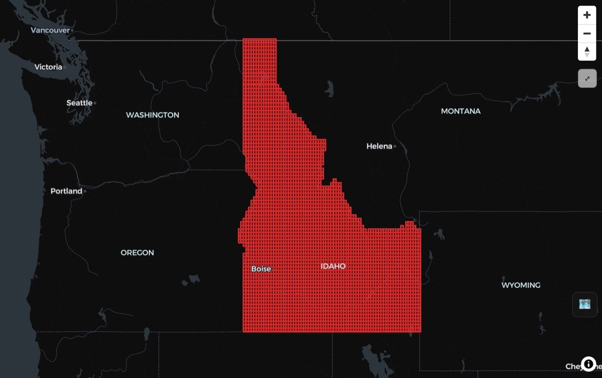
Raster data visualization: Land cover classification
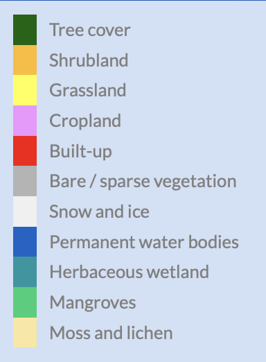
Now, let’s take a look at those land cover classifications! 😍RS_AsImage(rast, 300)→ Converts raster tiles to images.SedonaUtils.display_image()→ Displays raster images inline.