Private Preview
The following content is a read-only preview of an executable Jupyter notebook.To run this notebook interactively:
  1. Go to the Wherobots Model Hub.
  2. Select the specific notebook you wish to run.
  3. Click Run Model in Notebook.
This notebook will guide you through detecting field boundaries from satellite imagery, using Wherobots RasterFlow and the Fields of the World (FTW)1 model. You will gain a hands-on understanding of how to run models like Fields of the World on your selected area of interest, vectorize the model outputs, and work with those vectors in WherobotsDB.

Fields of the World (FTW)

The Fields of the World (FTW) model is an example of an open source segmentation model that can predict crop field boundaries. This model predicts 3 classes:
  • non_field_background
  • field
  • field_boundaries
It was trained on Sentinel-2 satellite imagery and labeled crop field data from 24 countries across 4 continents.

Inference on seasonal planting / harvest multi-spectral imagery

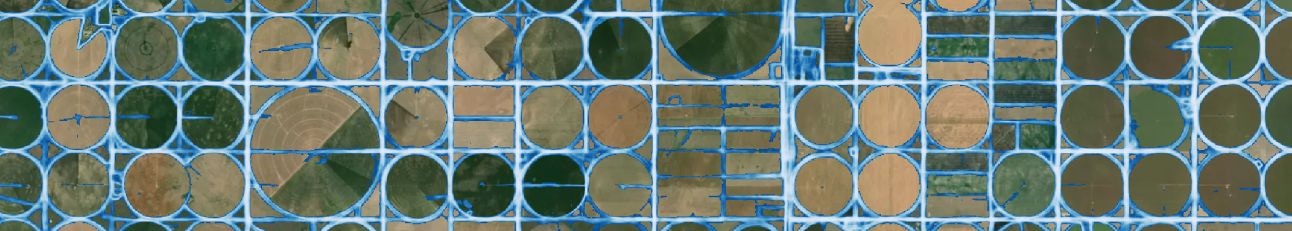
We’ll run the Fields of the World model on median pixel mosaics for the planting and harvest seasons using 4 multi-spectral bands for each season: Red, Green, Blue, and NIR. This data is sourced from Sentinel-2 L2A product2 from the European Space Agency. Rather than needing to create these mosaics manually, we’ll use RasterFlow’s registered datasets for Sentinel-2 seasonal mosaics, which are built in to this model recipe.

Selecting an Area of Interest (AOI)

To start, we will choose an Area of Interest (AOI) for our analysis. The area around Haskell County, Kansas has some interesting crop field patterns so we will try out the model there.
import wkls
import geopandas as gpd
import os

# Generate a geometry for Haskell County, Kansas using WKLS (https://github.com/wherobots/wkls)
gdf = gpd.read_file(wkls['us']['ks']['Haskell County'].geojson())

# Save the geometry to a parquet file in the user's S3 path
aoi_path = os.getenv("USER_S3_PATH") + "haskell.parquet"
gdf.to_parquet(aoi_path)

# Make variables for the bounds of our aoi for visualizing results after inference
min_lon, min_lat, max_lon, max_lat = gdf.total_bounds

Initializing the RasterFlow client

from datetime import datetime

from rasterflow_remote import RasterflowClient

from rasterflow_remote.data_models import (
    ModelRecipes, 
    VectorizeMethodEnum
)

rf_client = RasterflowClient()

Running a model

RasterFlow has pre-defined workflows to simplify orchestration of the processing steps for model inference. These steps include:
  • Ingesting imagery for the specified Area of Interest (AOI)
  • Generating a seamless image from multiple image tiles (a mosaic)
  • Running inference with the selected model
The output is a Zarr store of the model outputs. Note: This step will take approximately 30 minutes to complete.
model_outputs = rf_client.build_and_predict_mosaic_recipe(
    # Path to our AOI in GeoParquet or GeoJSON format
    aoi = aoi_path,

    # Date range for imagery to be used by the model
    start = datetime(2023, 1, 1),
    end = datetime(2024, 1, 1),

    # Coordinate Reference System EPSG code for the output mosaic   
    crs_epsg = 3857,

    # The model recipe to be used for inference (FTW in this case)
    model_recipe = ModelRecipes.FTW,
)

print(model_outputs)

Visualize a subset of the model outputs

The raster outputs from the model for this AOI are approximately 1GB. We can choose a small subset of the data around the Plymell, Kansas and use hvplot to visualize the model outputs.
# Import libraries for visualization and coordinate transformation
import hvplot.xarray
import xarray as xr
import s3fs 
import zarr
from pyproj import Transformer
from holoviews.element.tiles import EsriImagery 

# Open the Zarr store
fs = s3fs.S3FileSystem(profile="default", asynchronous=True)
zstore = zarr.storage.FsspecStore(fs, path=model_outputs[5:])
ds = xr.open_zarr(zstore)

# Create a transformer to convert from lat/lon to meters
transformer = Transformer.from_crs("EPSG:4326", "EPSG:3857", always_xy=True)

# Transform bounding box coordinates from lat/lon to meters
(min_x, max_x), (min_y, max_y) = transformer.transform(
    [min_lon, max_lon], 
    [min_lat, max_lat]
)

# Select the height variable and slice the dataset to the bounding box
# y=slice(max_y, min_y) handles the standard "North-to-South" image orientation
ds_subset = ds.sel(band="field_boundaries",
    x=slice(min_x, max_x), 
    y=slice(max_y, min_y) 
)

# Select the first time step and extract the variables array
arr_subset = ds_subset.isel(time=0)["variables"]

# Create a base map layer using Esri satellite imagery
base_map = EsriImagery()

# Create an overlay layer from the model outputs with hvplot
output_layer = arr_subset.hvplot(
    x = "x",
    y = "y",
    geo = True,           # Enable geographic plotting
    dynamic = True,       # Enable dynamic rendering for interactivity
    rasterize = True,     # Use datashader for efficient rendering of large datasets
    cmap = "viridis",     # Color map for visualization
    aspect = "equal",     # Maintain equal aspect ratio
    title = "FTW Model Outputs" 
).opts(
    width = 600, 
    height = 600,
    alpha = 0.7           # Set transparency to see the base map underneath
)

# Combine the base map and output layer
final_plot = base_map * output_layer
final_plot

Vectorize the raster model outputs

The output for the FTW model is a raster with three classes as bands: field, field_boundaries, and non_field_background. We will run a seperate flow to convert the fields and field boundaries into vector geometries. Converting these results to geometries allows us to more easily post process the results or join the results with other vector data.
# Determine the classes that are predicted by the model
model_features = xr.open_zarr(zstore)['band'].data.tolist()

# Remove the 'non_field_background' class for vectorization
vector_features = [f for f in model_features if f != 'non_field_background']    
# Note: this should take about 5 minutes to complete
vectorized_results = rf_client.vectorize_mosaic(
        store = model_outputs,
        features = vector_features,
        threshold = 0.5,
        vectorize_method = VectorizeMethodEnum.SEMANTIC_SEGMENTATION_RASTERIO,
        vectorize_config={"stats": True, "medial_skeletonize": False}
    )

print(vectorized_results)

Save the vectorized results to the catalog

We can store these vectorized outputs in the catalog by using WherobotsDB to persist the GeoParquet results.
from sedona.spark import *
config = SedonaContext.builder().getOrCreate()
sedona = SedonaContext.create(config)
sedona.sql("CREATE DATABASE IF NOT EXISTS org_catalog.ftw_db")

vectorize_result_df = sedona.read.format("geoparquet").load(vectorized_results)
vectorize_result_df = vectorize_result_df.withColumnRenamed("label", "layer")
vectorize_result_df.writeTo("org_catalog.ftw_db.ftw_vectorized").createOrReplace()

Visualize the vectorized results

To visualize the vectorized results, we will show the fields around Plymell, Kansas and filter out results with a score lower than 0.5. This threshold was determined through observation to strike a balance: it eliminates obvious noise without being overly aggressive, ensuring that we don’t accidentally filter out too many relevant results.
from sedona.spark.sql.st_constructors import ST_GeomFromText
from sedona.spark.sql.st_predicates import ST_Intersects
import pyspark.sql.functions as f

# Bounding box for Plymell, Kansas
plymell_wkt = "POLYGON ((-100.98 37.83, -100.98 37.68, -100.8 37.68, -100.8 37.83, -100.98 37.83))"
vectorize_result_filtered_df = vectorize_result_df.filter("layer == 'field'").filter("score_mean > 0.5") \
    .filter(ST_Intersects(f.col("geometry"), ST_GeomFromText(lit(plymell_wkt))))
We will apply some WherobotsDB vector post processing operations to refine the model results.
tolerance = 0.00001
decimal_places = 6  # roughly 10cm in lat/lon
df = vectorize_result_filtered_df.withColumn("geometry", f.expr("ST_MakeValid(geometry)"))
df = df.withColumn("geometry", f.expr("ST_SetSRID(geometry, 4326)")) # vectorize_mosaic defaults to returning geometries in the CRS EPSG:4326
df = df.withColumn("geometry", f.expr(f"ST_ReducePrecision(geometry, {decimal_places})"))
df = df.withColumn("geometry", f.expr(f"ST_SimplifyPreserveTopology(geometry, {tolerance})"))
df = df.repartition(200)
df.show()
from sedona.spark.maps.SedonaKepler import SedonaKepler
map = SedonaKepler.create_map(df=df, name="Vectorized results")
map

Generate PM Tiles for visualization

To improve visualization performance of a large number of geometries, we can use Wherobots built-in high performance PM tile generator. The FTW model has a tendency to create extremely large boundary geometries, which doesn’t play nicely with PMTiles. To avoid this we subdivide the boundary geometries.
fields_df = df.where("layer = 'field'")
# 1266 is the vertex count of the second-largest boundary geometry.
# We use this instead of the absolute largest boundary (an extreme outlier)
# so the subdivision threshold is high enough to keep most geometries intact
# while still forcing that outlier-sized boundary to be subdivided for
# better PMTiles rendering performance.
boundaries_df = df.where("layer = 'field_boundaries'").withColumn("geometry", f.expr("ST_SubDivideExplode(geometry, 1266)"))
tile_features_df = fields_df.withColumn("layer", f.lit("fields")).unionByName(
    boundaries_df.withColumn("layer", f.lit("boundaries"))
)
from wherobots import vtiles
full_tiles_path = os.getenv("USER_S3_PATH") + "tiles.pmtiles"
vtiles.generate_pmtiles(tile_features_df, full_tiles_path)
vtiles.show_pmtiles(full_tiles_path)

Sharing PMTiles results with the Wherobots PMTiles Viewer

You can generate a pre-signed url to your pmtiles using get_url. Then, copy this to your clipboard with right-click + “Copy Output to Clipboard”. You can paste this url into https://tile-viewer.wherobots.com/ and create a publicly accessible PMTiles map served from your own bucket.
from wherobots.tools.utility.s3_utils import get_url

get_url(full_tiles_path)

References

  1. Kerner, H., Chaudhari, S., Ghosh, A., Robinson, C., Ahmad, A., Choi, E., Jacobs, N., Holmes, C., Mohr, M., et al. (2024). Fields of The World: A Machine Learning Benchmark Dataset For Global Agricultural Field Boundary Segmentation. arXiv preprint arXiv:2409.16252. Accepted at AAAI-2025 Artificial Intelligence for Social Impact (AISI) track.
  2. ESA. (2015). Sentinel-2 User Handbook (Issue 1, Rev. 2). European Space Agency. https://sentinels.copernicus.eu/documents/247904/685211/Sentinel-2_User_Handbook