Private Preview
The following content is a read-only preview of an executable Jupyter notebook.To run this notebook interactively:
  1. Go to the Wherobots Model Hub.
  2. Select the specific notebook you wish to run.
  3. Click Run Model in Notebook.
This notebook will guide you through estimating canopy height from aerial imagery, using Wherobots RasterFlow and the Meta and World Resources Institute’s Canopy Height prediction model (Meta CHM v1)1. This is an open source regression model that can predict the height of the tree canopy from high resolution imagery. The result of the model is a raster where each pixel is the estimated tree canopy height in meters. It was trained on high-resoluton imagery (Maxar Vivid2 mosaic with 0.5m resolution), existing labeled canopy height maps and airborne laser scans (LIDAR).

Running inference on high resolution imagery

The Meta CHM v1 model was trained on 50cm resolution data, so we will select imagery with a similar resolution for our testing. The National Agriculture Imagery Program (NAIP) provides aerial imagery for the United States, capturing high-resolution images during the agricultural growing seasons. The NAIP dataset contains a mixture of resolutions (30cm, 60cm and 1m). See this map for more details. We will use 60cm imagery to test this model.

Selecting an Area of Interest (AOI)

We will choose an Area of Interest (AOI) for our analysis. The area around Nashua, NH has a combination of urban settings, parks and forests so we will try out the model there. From the map, we see that 60cm imagery for New Hampshire was last captured in 2021, so we will set our time range accordingly.
import wkls
import geopandas as gpd
import os

# Generate a geometry for Nashua, NH using WKLS (https://github.com/wherobots/wkls)
gdf = gpd.read_file(wkls.us.nh.nashua.geojson())

# Save the geometry to a parquet file in the user's S3 path
aoi_path = os.getenv("USER_S3_PATH") + "nashua.parquet"
gdf.to_parquet(aoi_path)

# we'll make variables for the bounds of our aoi for use after running inference to visualize results
min_lon, min_lat, max_lon, max_lat = gdf.total_bounds

Initializing the RasterFlow client

from datetime import datetime

from rasterflow_remote import RasterflowClient

from rasterflow_remote.data_models import (
    ModelRecipes
)

rf_client = RasterflowClient()

Running a model

RasterFlow has pre-defined workflows to simplify orchestration of the processing steps for model inference. These steps include:
  • Ingesting imagery for the specified Area of Interest (AOI)
  • Generating a seamless image from multiple image tiles (a mosaic)
  • Running inference with the selected model
The output is a Zarr store of the model outputs. Note: This step will take approximately 20 minutes to complete.
model_outputs = rf_client.build_and_predict_mosaic_recipe(
    # Path to our AOI in GeoParquet or GeoJSON format
    aoi = aoi_path,

    # Date range for imagery to be used by the model
    start = datetime(2021, 1, 1),
    end = datetime(2022, 1, 1),

    # Coordinate Reference System EPSG code for the output mosaic   
    crs_epsg = 3857,

    # The model recipe to be used for inference (CHM in this case)
    model_recipe = ModelRecipes.META_CHM_V1
)

print(model_outputs)

Visualize a subset of the model outputs

We will use hvplot and datashader to visualize a small subset of the model outputs.
# Import libraries for visualization and coordinate transformation
import hvplot.xarray
import xarray as xr
import s3fs 
import zarr
from pyproj import Transformer
from holoviews.element.tiles import EsriImagery 

# Open the Zarr store
fs = s3fs.S3FileSystem(profile="default", asynchronous=True)
zstore = zarr.storage.FsspecStore(fs, path=model_outputs[5:])
ds = xr.open_zarr(zstore)

# Create a transformer to convert from lat/lon to meters
transformer = Transformer.from_crs("EPSG:4326", "EPSG:3857", always_xy=True)

# Transform bounding box coordinates from lat/lon to meters
(min_x, max_x), (min_y, max_y) = transformer.transform(
    [min_lon, max_lon], 
    [min_lat, max_lat]
)

# Select the height variable and slice the dataset to the bounding box
# y=slice(max_y, min_y) handles the standard "North-to-South" image orientation
ds_subset = ds.sel(band="height",
    x=slice(min_x, max_x), 
    y=slice(max_y, min_y) 
)

# Select the first time step and extract the variables array
arr_subset = ds_subset.isel(time=0)["variables"]

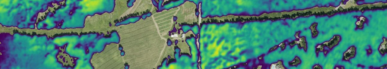
# Create a base map layer using Esri satellite imagery
base_map = EsriImagery()

# Create an overlay layer from the model outputs with hvplot
output_layer = arr_subset.hvplot(
    x = "x",
    y = "y",
    geo = True,           # Enable geographic plotting
    dynamic = True,       # Enable dynamic rendering for interactivity
    rasterize = True,     # Use datashader for efficient rendering of large datasets
    cmap = "viridis",     # Color map for visualization
    aspect = "equal",     # Maintain equal aspect ratio
    title = "CHM Model Outputs" 
).opts(
    width = 600, 
    height = 600,
    alpha = 0.7           # Set transparency to see the base map underneath
)

# Combine the base map and output layer
final_plot = base_map * output_layer
final_plot

References

  1. Tolan, J., Yang, H.-I., Nosarzewski, B., Couairon, G., Vo, H. V., Brandt, J., Spore, J., Majumdar, S., Haziza, D., Vamaraju, J., et al. (2024). Very high resolution canopy height maps from RGB imagery using self-supervised vision transformer and convolutional decoder trained on aerial lidar. Remote Sensing of Environment, 300, 113888.