The following content is a read-only preview of an executable Jupyter notebook.To run this notebook interactively:
  1. Go to Wherobots Cloud.
  2. Start a runtime.
  3. Open the notebook.
  4. In the Jupyter Launcher:
    1. Click File > Open Path.
    2. Paste the following path to access this notebook: examples/Open_Data_Connections/ESA_WorldCover.ipynb
    3. Click Enter.
This notebook introduces ESA WorldCover raster data in Wherobots. We will:
  • Load Cloud Optimized GeoTIFF (COG) rasters from ESA WorldCover on AWS S3.
  • Use Wherobots to explore raster metadata and perform spatial filtering.
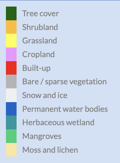
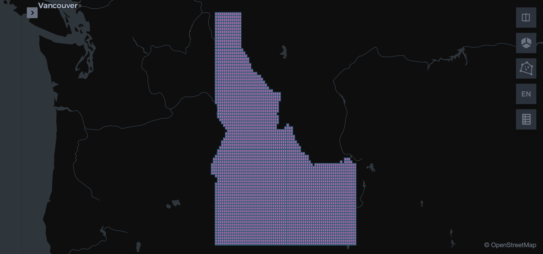
  • Visualize tile distributions and land cover classifications over Idaho.

Why Use Wherobots for ESA WorldCover?

Processing large-scale raster data is often slow and memory-intensive. With Wherobots, we leverage:
  • Lazy loading: raster data is not pulled into memory until needed.
  • Distributed raster access: fast indexing and querying without moving large files.
  • Optimized COG reads: only necessary raster tiles are accessed.
  • Integrated raster + vector operations: spatial joins across data types in one environment.
You can overlay ESA WorldCover rasters with:
  • Vector boundaries (e.g., administrative regions, watersheds)
  • Point datasets (e.g., GPS locations, sensor data)
  • Line features (e.g., roads, rivers)
This enables efficient exploration and analysis before deeper processing.

What is ESA WorldCover?

The ESA WorldCover dataset provides high-resolution global land cover maps developed using Sentinel-1 & Sentinel-2 satellite imagery.

How is This Useful?

This dataset allows us to analyze land cover changes for:
  • Urban expansion: Identifying areas undergoing rapid development.
  • Monitoring deforestation: Detecting changes in forest cover over time.
  • Water body analysis: Observing changes in lakes, rivers, and coastal areas.
  • Agriculture and land use: Mapping croplands and classifying vegetation.

Dataset overview

  • Resolution: 10 meters
  • Years available: 2020, 2021
  • Format**: Cloud Optimized GeoTIFF (COG)**
  • Hosted on AWS: s3://esa-worldcover/v200/2021/map/
  • Projectio: EPSG:4326 (WGS84 or Web Mercator)
With Wherobots, we can quickly access and filter this dataset and perform detailed analyses.

Set up the Sedona context

from sedona.spark import *

try:
    sedona
except NameError:
    config = SedonaContext.builder() \
        .getOrCreate()
    sedona = SedonaContext.create(config)

Raster data sources in Wherobots

Wherobots provides a powerful raster data source that allows users to:
  • Read Cloud Optimized GeoTIFFs (COGs) efficiently in a distributed manner.
  • Dynamically tile large rasters for parallel processing across multiple nodes.
  • Perform spatial filtering before pixel processing, improving performance.

Why retiling matters

Retiling helps:
  • Optimize query performance by breaking large images into manageable chunks.
  • Speed up spatial joins and filtering, as each tile is processed independently.
  • Reduce memory overhead, ensuring raster operations are efficient.
If you prefer to work with the original raster structure, you can disable retiling using: option("retile", "false")
df2 = sedona.read.format("raster").option("retile", "true").load("s3://esa-worldcover/v200/2021/map/*.tif*")
df2.printSchema()
df2.count()

Understanding raster metadata

Before processing rasters, it is useful to inspect its metadata:
  • Geometry (RS_Envelope): The spatial extent of each raster tile.
  • Area (ST_Area): The real-world area covered by each tile.
  • Metadata (RS_Metadata): All metadata of the raster including tile size, coordinate reference system, etc. Documentation on the metadata for rasters.
These allow us to spatially filter and query raster data efficiently.
from pyspark.sql.functions import col, expr

esa_df = df2.withColumn("geometry", expr("RS_Envelope(rast)"))\
            .withColumn("area", expr("ST_Area(geometry)"))\
            .withColumn("metadata", expr("RS_Metadata(rast)"))
esa_df.show()

Exploring Idaho’s land cover tiles

Let’s explore the ESA WorldCover land cover tiles in Idaho** and see how they look.
Using the ST_Intersects predicate, we can filter the raster tiles that intersect with the Idaho state boundary.
Since Wherobots lazy loads raster data, this operation only filters metadata without actually loading raster pixels, helping ensure optimal performance.
idaho_wkt = 'POLYGON ((-117.025719 42.008404, -111.038632 42.008404, -111.049617 44.457228, -111.379182 44.738848, -111.489037 44.652943, -111.423124 44.535593, -111.653819 44.574736, -111.818601 44.519928, -112.279991 44.551253, -112.785323 44.480748, -112.829265 44.34734, -113.005033 44.527761, -113.103902 44.738848, -113.257699 44.816834, -113.411496 44.855787, -113.496919 44.945341, -113.450231 44.951173, -113.433753 45.007515, -113.455724 45.061861, -113.521637 45.085137, -113.502412 45.116156, -113.565578 45.120033, -113.562832 45.158781, -113.680926 45.274866, -113.7386 45.325096, -113.733107 45.390715, -113.777049 45.41, -113.760571 45.481298, -113.763317 45.517875, -113.82923 45.519799, -113.790781 45.587114, -113.815498 45.615938, -113.897889 45.619781, -113.881411 45.650508, -113.936338 45.700405, -113.991266 45.709995, -114.032461 45.683138, -114.013237 45.650508, -114.059925 45.635147, -114.128584 45.58327, -114.153302 45.556352, -114.252171 45.550582, -114.337308 45.462037, -114.367519 45.498627, -114.422446 45.514026, -114.455402 45.565967, -114.551525 45.565967, -114.529554 45.60441, -114.557018 45.635147, -114.493852 45.665866, -114.491105 45.708077, -114.559764 45.77325, -114.499344 45.836434, -114.414207 45.847914, -114.38125 45.886165, -114.427939 45.935851, -114.397729 45.960677, -114.427939 45.995034, -114.474627 46.000758, -114.466388 46.027462, -114.502091 46.036996, -114.452656 46.096071, -114.521315 46.145569, -114.438924 46.166497, -114.441671 46.236833, -114.469134 46.274815, -114.425192 46.278611, -114.4197 46.310873, -114.405968 46.356387, -114.416953 46.381024, -114.367519 46.441622, -114.400475 46.490809, -114.342801 46.511606, -114.323577 46.577723, -114.32083 46.658843, -114.359279 46.675806, -114.422446 46.664498, -114.458149 46.655072, -114.477373 46.634331, -114.546033 46.655072, -114.603706 46.639988, -114.609199 46.660728, -114.617438 46.709716, -114.647648 46.737959, -114.699829 46.749251, -114.724547 46.719132, -114.773981 46.715366, -114.75201 46.75866, -114.78222 46.786877, -114.861865 46.818838, -114.927778 46.860171, -114.914046 46.920236, -114.996437 46.980233, -115.136502 47.100025, -115.257342 47.182226, -115.320509 47.260573, -115.52374 47.301565, -115.540219 47.357412, -115.611624 47.390892, -115.746196 47.42621, -115.611624 47.481925, -115.691269 47.533873, -115.685776 47.596884, -115.71324 47.702349, -115.787392 47.757772, -115.856051 47.83342, -116.048297 47.982549, -116.045551 49.001825, -117.028751 49.000023, -117.035969 46.445348, -116.9371 46.172143, -117.003013 46.07315, -116.47571 45.606271, -117.266664 44.441542, -117.233708 44.292318, -116.948085 44.166362, -117.035969 43.834444, -117.025719 42.008404))'
# Filter Idaho land cover tiles
idaho_df = esa_df.filter(f"ST_Intersects(geometry, ST_GeomFromWKT('{idaho_wkt}'))")

idaho_df.count()

Visualize the spatial extent of the tiles

SedonaKepler.create_map(idaho_df.select("geometry"))
image.png

Raster data visualization: Land cover classification

Now, let’s take a look at those land cover classifications! 😍
  • RS_AsImage(rast, 300) → Converts raster tiles to images.
  • SedonaUtils.display_image() → Displays raster images inline.
image.png
htmlDf = idaho_df.selectExpr("RS_AsImage(rast, 300)").limit(5)
SedonaUtils.display_image(htmlDf)