Optimizers

Sedona Spatial operators fully supports Apache SparkSQL query optimizer. It has the following query optimization features:

Automatically optimizes range join query and distance join query.
Automatically performs predicate pushdown.

Sedona join performance is heavily affected by the number of partitions. If the join performance is not ideal, please increase the number of partitions by doing df.repartition(XXX) right after you create the original DataFrame.

Range join

Introduction: Find geometries from A and geometries from B such that each geometry pair satisfies a certain predicate. Most predicates supported by Spatial SQL can trigger a range join. SQL example:

SELECT *
FROM polygondf, pointdf
WHERE ST_Contains(polygondf.polygonshape,pointdf.pointshape)

SELECT *
FROM polygondf, pointdf
WHERE ST_Intersects(polygondf.polygonshape,pointdf.pointshape)

SELECT *
FROM pointdf, polygondf
WHERE ST_Within(pointdf.pointshape, polygondf.polygonshape)

SELECT *
FROM pointdf, polygondf
WHERE ST_DWithin(pointdf.pointshape, polygondf.polygonshape, 10.0)

Spark SQL Physical plan:

== Physical Plan ==
RangeJoin polygonshape#20: geometry, pointshape#43: geometry, false
:- Project [st_polygonfromenvelope(cast(_c0#0 as decimal(24,20)), cast(_c1#1 as decimal(24,20)), cast(_c2#2 as decimal(24,20)), cast(_c3#3 as decimal(24,20)), mypolygonid) AS polygonshape#20]
:  +- *FileScan csv
+- Project [st_point(cast(_c0#31 as decimal(24,20)), cast(_c1#32 as decimal(24,20)), myPointId) AS pointshape#43]
   +- *FileScan csv

Distance join

Introduction: Find geometries from A and geometries from B such that the distance of each geometry pair is less or equal than a certain distance. It supports the planar Euclidean distance calculators ST_Distance, ST_HausdorffDistance, ST_FrechetDistance and the meter-based geodesic distance calculators ST_DistanceSpheroid and ST_DistanceSphere. SQL example for planar Euclidean distance: Only consider

SELECT *
FROM pointdf1, pointdf2
WHERE ST_Distance(pointdf1.pointshape1,pointdf2.pointshape2) < 2

SELECT *
FROM pointDf, polygonDF
WHERE ST_HausdorffDistance(pointDf.pointshape, polygonDf.polygonshape, 0.3) < 2

SELECT *
FROM pointDf, polygonDF
WHERE ST_FrechetDistance(pointDf.pointshape, polygonDf.polygonshape) < 2

Consider

SELECT *
FROM pointdf1, pointdf2
WHERE ST_Distance(pointdf1.pointshape1,pointdf2.pointshape2) <= 2

SELECT *
FROM pointDf, polygonDF
WHERE ST_HausdorffDistance(pointDf.pointshape, polygonDf.polygonshape) <= 2

SELECT *
FROM pointDf, polygonDF
WHERE ST_FrechetDistance(pointDf.pointshape, polygonDf.polygonshape) <= 2

SQL Physical plan:

== Physical Plan ==
DistanceJoin pointshape1#12: geometry, pointshape2#33: geometry, 2.0, true
:- Project [st_point(cast(_c0#0 as decimal(24,20)), cast(_c1#1 as decimal(24,20)), myPointId) AS pointshape1#12]
:  +- *FileScan csv
+- Project [st_point(cast(_c0#21 as decimal(24,20)), cast(_c1#22 as decimal(24,20)), myPointId) AS pointshape2#33]
   +- *FileScan csv

If you use planar euclidean distance functions like ST_Distance, ST_HausdorffDistance or ST_FrechetDistance as the predicate, Sedona doesn’t control the distance’s unit (degree or meter). It is same with the geometry. If your coordinates are in the longitude and latitude system, the unit of distance should be degree instead of meter or mile. To change the geometry’s unit, please either transform the coordinate reference system to a meter-based system. See CRS Transformation. If you don’t want to transform your data, please consider using ST_DistanceSpheroid or ST_DistanceSphere.

SQL example for meter-based geodesic distance ST_DistanceSpheroid (works for ST_DistanceSphere too): Less than a certain distance==

SELECT *
FROM pointdf1, pointdf2
WHERE ST_DistanceSpheroid(pointdf1.pointshape1,pointdf2.pointshape2) < 2

Less than or equal to a certain distance==

SELECT *
FROM pointdf1, pointdf2
WHERE ST_DistanceSpheroid(pointdf1.pointshape1,pointdf2.pointshape2) <= 2

If you use ST_DistanceSpheroid or ST_DistanceSphere as the predicate, the unit of the distance is meter. Currently, distance join with geodesic distance calculators work best for point data. For non-point data, it only considers their centroids.

Broadcast index join

Introduction: Perform a range join or distance join but broadcast one of the sides of the join. This maintains the partitioning of the non-broadcast side and doesn’t require a shuffle. Sedona will create a spatial index on the broadcasted table. Sedona uses broadcast join only if the correct side has a broadcast hint. The supported join type - broadcast side combinations are:

Inner - either side, preferring to broadcast left if both sides have the hint
Left semi - broadcast right
Left anti - broadcast right
Left outer - broadcast right
Right outer - broadcast left

pointDf.alias("pointDf").join(broadcast(polygonDf).alias("polygonDf"), expr("ST_Contains(polygonDf.polygonshape, pointDf.pointshape)"))

SQL Physical plan:

== Physical Plan ==
BroadcastIndexJoin pointshape#52: geometry, BuildRight, BuildRight, false ST_Contains(polygonshape#30, pointshape#52)
:- Project [st_point(cast(_c0#48 as decimal(24,20)), cast(_c1#49 as decimal(24,20))) AS pointshape#52]
:  +- FileScan csv
+- SpatialIndex polygonshape#30: geometry, QUADTREE, [id=#62]
   +- Project [st_polygonfromenvelope(cast(_c0#22 as decimal(24,20)), cast(_c1#23 as decimal(24,20)), cast(_c2#24 as decimal(24,20)), cast(_c3#25 as decimal(24,20))) AS polygonshape#30]
      +- FileScan csv

This also works for distance joins with ST_Distance, ST_DistanceSpheroid, ST_DistanceSphere, ST_HausdorffDistance or ST_FrechetDistance:

pointDf1.alias("pointDf1").join(broadcast(pointDf2).alias("pointDf2"), expr("ST_Distance(pointDf1.pointshape, pointDf2.pointshape) <= 2"))

SQL Physical plan:

== Physical Plan ==
BroadcastIndexJoin pointshape#52: geometry, BuildRight, BuildLeft, true, 2.0 ST_Distance(pointshape#52, pointshape#415) <= 2.0
:- Project [st_point(cast(_c0#48 as decimal(24,20)), cast(_c1#49 as decimal(24,20))) AS pointshape#52]
:  +- FileScan csv
+- SpatialIndex pointshape#415: geometry, QUADTREE, [id=#1068]
   +- Project [st_point(cast(_c0#48 as decimal(24,20)), cast(_c1#49 as decimal(24,20))) AS pointshape#415]
      +- FileScan csv

Note: If the distance is an expression, it is only evaluated on the first argument to ST_Distance (pointDf1 above).

Automatic broadcast index join

When one table involved a spatial join query is smaller than a threshold, Sedona will automatically choose broadcast index join instead of Sedona optimized join. The current threshold is controlled by sedona.join.autoBroadcastJoinThreshold and set to the same as spark.sql.autoBroadcastJoinThreshold.

Raster join

The optimization for spatial join also works for raster predicates, such as RS_Intersects, RS_Contains and RS_Within. SQL Example:

-- Raster-geometry join
SELECT df1.id, df2.id, RS_Value(df1.rast, df2.geom) FROM df1 JOIN df2 ON RS_Intersects(df1.rast, df2.geom)

-- Raster-raster join
SELECT df1.id, df2.id FROM df1 JOIN df2 ON RS_Intersects(df1.rast, df2.rast)

These queries could be planned as RangeJoin or BroadcastIndexJoin. Here is an example of the physical plan using RangeJoin:

== Physical Plan ==
*(1) Project [id#14, id#25]
+- RangeJoin rast#13: raster, geom#24: geometry, INTERSECTS,  **org.apache.spark.sql.sedona_sql.expressions.RS_Intersects**
   :- LocalTableScan [rast#13, id#14]
   +- LocalTableScan [geom#24, id#25]

Google S2 based approximate equi-join

If the performance of Sedona optimized join is not ideal, which is possibly caused by complicated and overlapping geometries, you can resort to Sedona built-in Google S2-based approximate equi-join. This equi-join leverages Spark’s internal equi-join algorithm and might be performant given that you can opt to skip the refinement step by sacrificing query accuracy. Please use the following steps:

1. Generate S2 ids for both tables

Use ST_S2CellIds to generate cell IDs. Each geometry may produce one or more IDs.

SELECT id, geom, name, explode(ST_S2CellIDs(geom, 15)) as cellId
FROM lefts

SELECT id, geom, name, explode(ST_S2CellIDs(geom, 15)) as cellId
FROM rights

2. Perform equi-join

Join the two tables by their S2 cellId

SELECT lcs.id as lcs_id, lcs.geom as lcs_geom, lcs.name as lcs_name, rcs.id as rcs_id, rcs.geom as rcs_geom, rcs.name as rcs_name
FROM lcs JOIN rcs ON lcs.cellId = rcs.cellId

3. Optional: Refine the result

Due to the nature of S2 Cellid, the equi-join results might have a few false-positives depending on the S2 level you choose. A smaller level indicates bigger cells, less exploded rows, but more false positives. To ensure the correctness, you can use one of the Spatial Predicates to filter out them. Use this query instead of the query in Step 2.

SELECT lcs.id as lcs_id, lcs.geom as lcs_geom, lcs.name as lcs_name, rcs.id as rcs_id, rcs.geom as rcs_geom, rcs.name as rcs_name
FROM lcs, rcs
WHERE lcs.cellId = rcs.cellId AND ST_Contains(lcs.geom, rcs.geom)

As you see, compared to the query in Step 2, we added one more filter, which is ST_Contains, to remove false positives. You can also use ST_Intersects and so on.

You can skip this step if you don’t need 100% accuracy and want faster query speed.

4. Optional: De-duplicate

Due to the explode function used when we generate S2 Cell Ids, the resulting DataFrame may have several duplicate <lcs_geom, rcs_geom> matches. You can remove them by performing a GroupBy query.

SELECT lcs_id, rcs_id, first(lcs_geom), first(lcs_name), first(rcs_geom), first(rcs_name)
FROM joinresult
GROUP BY (lcs_id, rcs_id)

The first function is to take the first value from a number of duplicate values. If you don’t have a unique id for each geometry, you can also group by geometry itself. See below:

SELECT lcs_geom, rcs_geom, first(lcs_name), first(rcs_name)
FROM joinresult
GROUP BY (lcs_geom, rcs_geom)

If you are doing point-in-polygon join, this is not a problem and you can safely discard this issue. This issue only happens when you do polygon-polygon, polygon-linestring, linestring-linestring join.

S2 for distance join

This also works for distance join. You first need to use ST_Buffer(geometry, distance) to wrap one of your original geometry column. If your original geometry column contains points, this ST_Buffer will make them become circles with a radius of distance. Since the coordinates are in the longitude and latitude system, so the unit of distance should be degree instead of meter or mile. You can get an approximation by performing METER_DISTANCE/111000.0, then filter out false-positives. Note that this might lead to inaccurate results if your data is close to the poles or antimeridian. In a nutshell, run this query first on the left table before Step 1. Please replace METER_DISTANCE with a meter distance. In Step 1, generate S2 IDs based on the buffered_geom column. Then run Step 2, 3, 4 on the original geom column.

SELECT id, geom, ST_Buffer(geom, METER_DISTANCE/111000.0) as buffered_geom, name
FROM lefts

Regular spatial predicate pushdown

Introduction: Given a join query and a predicate in the same WHERE clause, first executes the Predicate as a filter, then executes the join query. SQL example:

SELECT *
FROM polygondf, pointdf
WHERE ST_Contains(polygondf.polygonshape,pointdf.pointshape)
AND ST_Contains(ST_PolygonFromEnvelope(1.0,101.0,501.0,601.0), polygondf.polygonshape)

SQL Physical plan:

== Physical Plan ==
RangeJoin polygonshape#20: geometry, pointshape#43: geometry, false
:- Project [st_polygonfromenvelope(cast(_c0#0 as decimal(24,20)), cast(_c1#1 as decimal(24,20)), cast(_c2#2 as decimal(24,20)), cast(_c3#3 as decimal(24,20)), mypolygonid) AS polygonshape#20]
:  +- Filter  **org.apache.spark.sql.sedona_sql.expressions.ST_Contains$**
:     +- *FileScan csv
+- Project [st_point(cast(_c0#31 as decimal(24,20)), cast(_c1#32 as decimal(24,20)), myPointId) AS pointshape#43]
   +- *FileScan csv

Push spatial predicates to GeoParquet

Sedona supports spatial predicate push-down for GeoParquet files. When spatial filters were applied to dataframes backed by GeoParquet files, Sedona will use the bbox properties in the metadata to determine if all data in the file will be discarded by the spatial predicate. This optimization could reduce the number of files scanned when the queried GeoParquet dataset was partitioned by spatial proximity. To maximize the performance of Sedona GeoParquet filter pushdown, we suggest that you sort the data by their geohash values (see ST_GeoHash) and then save as a GeoParquet file. An example is as follows:

SELECT col1, col2, geom, ST_GeoHash(geom, 5) as geohash
FROM spatialDf
ORDER BY geohash

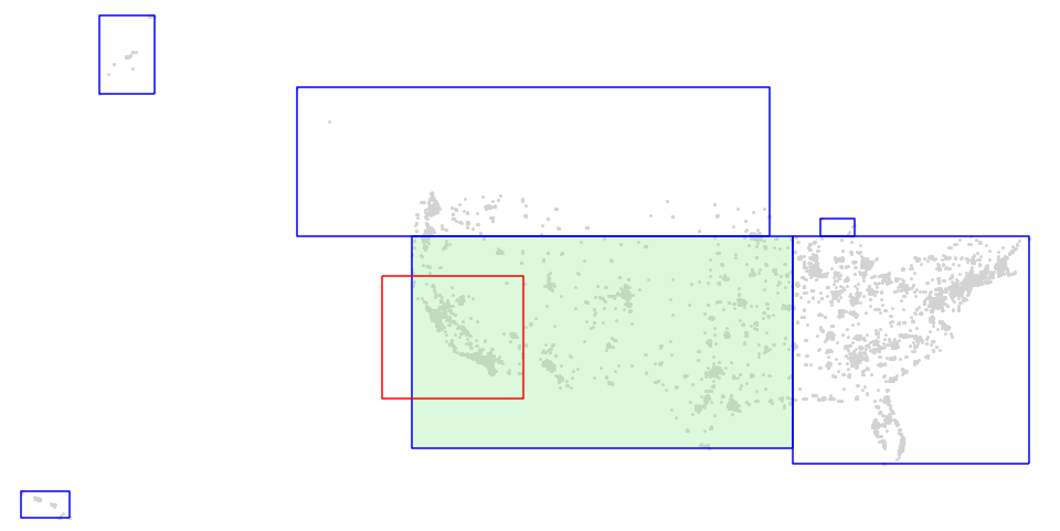
The following figure is the visualization of a GeoParquet dataset. bboxes of all GeoParquet files were plotted as blue rectangles and the query window was plotted as a red rectangle. Sedona will only scan 1 of the 6 files to answer queries such as SELECT * FROM geoparquet_dataset WHERE ST_Intersects(geom, <query window>), thus only part of the data covered by the light green rectangle needs to be scanned.

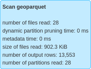
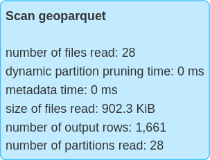
We can compare the metrics of querying the GeoParquet dataset with or without the spatial predicate and observe that querying with spatial predicate results in fewer number of rows scanned.

Without spatial predicate	With spatial predicate

Spatial predicate push-down to GeoParquet is enabled by default. Users can manually disable it by setting the Spark configuration spark.sedona.geoparquet.spatialFilterPushDown to false.

Box2D filter pushdown

When a query filters on a Box2D-typed column (see Box2D Functions) using ST_Intersects or ST_Contains against a literal Box2D, Sedona translates the predicate into Parquet row-group inequalities on the column’s underlying xmin / ymin / xmax / ymax leaves and pushes them down via ParquetInputFormat.setFilterPredicate. Parquet’s row-group statistics machinery then skips row groups whose recorded min/max disprove the predicate — no file metadata scan is required. The pushdown applies whenever the column’s Spark dataType is Box2DUDT. The simplest way to get one is to materialize the column with ST_Box2D(geom) before writing the dataset, or to use the SQL cast CAST(geom AS box2d). Sedona’s auto-generated <geom>_bbox covering column is written as a plain struct<xmin, ymin, xmax, ymax> — it satisfies the GeoParquet 1.1 covering-bbox contract but is not a Box2D, so ST_Intersects / ST_Contains do not target it directly. Use it through Push spatial predicates to GeoParquet (which prunes via the file-level bbox metadata), or write the column explicitly as ST_Box2D(geom) if you want row-group-level pruning through Box2D predicates.

SELECT *
FROM geoparquet_dataset
WHERE ST_Intersects(
    geom_bbox,
    ST_MakeBox2D(ST_Point(0.0, 0.0), ST_Point(10.0, 10.0)))

Predicate types and the per-row inequality system they translate to:

Predicate	Pushed-down conjunction (per row)
`ST_Intersects(box_col, lit)`	`box.xmax >= lit.xmin AND box.xmin <= lit.xmax AND box.ymax >= lit.ymin AND box.ymin <= lit.ymax` (symmetric — reverse arg order is identical)
`ST_Contains(box_col, lit)`	`box.xmin <= lit.xmin AND box.xmax >= lit.xmax AND box.ymin <= lit.ymin AND box.ymax >= lit.ymax`
`ST_Contains(lit, box_col)`	`box.xmin >= lit.xmin AND box.xmax <= lit.xmax AND box.ymin >= lit.ymin AND box.ymax <= lit.ymax`

Pushdown is enabled by default and is gated by two flags. The optimizer rule that attaches the Box2D spatial filter is controlled by spark.sedona.geoparquet.spatialFilterPushDown (Sedona’s master spatial-pushdown toggle, default true); the actual injection into the Parquet read path is then additionally gated by Spark’s spark.sql.parquet.filterPushdown (default true). Disabling either disables Box2D pushdown. Inverted-bound literals (xmin > xmax / ymin > ymax) are not pushed down — the predicate falls back to per-row evaluation so callers see the expected IllegalArgumentException from the scalar contract.

Box2D spatial join

ST_Intersects and ST_Contains between two Box2D columns route through the same physical operators as their Geometry counterparts (ST_Intersects / ST_Covers). At the executor boundary, each Box2D row is materialized into the implied rectangular polygon, after which the partitioner, R-tree index, and refine evaluator run unchanged. JTS short-circuits axis-aligned rectangle predicates via RectangleIntersects / RectangleContains, so the refine step pays only the four-double envelope comparison. ST_Contains uses SpatialPredicate.COVERS semantics at the join layer — JTS covers matches ST_Contains’s closed-interval contract (JTS contains, strict-interior, would reject edge-sharing pairs). Range join:

SELECT *
FROM left_boxes L, right_boxes R
WHERE ST_Intersects(L.box, R.box)

Broadcast index join:

SELECT /*+ BROADCAST(R) */ *
FROM left_boxes L, right_boxes R
WHERE ST_Intersects(L.box, R.box)

Inverted-bound input on either side raises IllegalArgumentException from the join-side validation path, matching the scalar predicate contract.

Wherobots Cloud REST API

WherobotsDB

Vector tiles (PMTiles)

Havasu (Iceberg) table management

GeoStats and Map Matching

Rasterflow

Range join

Distance join

Broadcast index join

Automatic broadcast index join

Raster join

Google S2 based approximate equi-join

1. Generate S2 ids for both tables

2. Perform equi-join

3. Optional: Refine the result

4. Optional: De-duplicate

S2 for distance join

Regular spatial predicate pushdown

Push spatial predicates to GeoParquet

Box2D filter pushdown

Box2D spatial join

​Range join

​Distance join

​Broadcast index join

​Automatic broadcast index join

​Raster join

​Google S2 based approximate equi-join

​1. Generate S2 ids for both tables

​2. Perform equi-join

​3. Optional: Refine the result

​4. Optional: De-duplicate

​S2 for distance join

​Regular spatial predicate pushdown

​Push spatial predicates to GeoParquet

​Box2D filter pushdown

​Box2D spatial join

Range join

Distance join

Broadcast index join

Automatic broadcast index join

Raster join

Google S2 based approximate equi-join

1. Generate S2 ids for both tables

2. Perform equi-join

3. Optional: Refine the result

4. Optional: De-duplicate

S2 for distance join

Regular spatial predicate pushdown

Push spatial predicates to GeoParquet

Box2D filter pushdown

Box2D spatial join