> ## Documentation Index
> Fetch the complete documentation index at: https://docs.wherobots.com/llms.txt
> Use this file to discover all available pages before exploring further.
# Raster Data in WherobotsDB
A raster is a regular grid of numeric values with geo-referencing metadata that describes the location and resolution of the grid. Raster data is commonly used to represent terrain, elevation, and satellite imagery. Havasu supports raster data type and allows users to store and query raster data. This tutorial describes how to use raster data type and raster functions in WherobotsDB for manipulating raster data.
## In-DB raster vs. Out-DB raster
WherobotsDB supports two types of raster data: In-DB raster and Out-DB raster. In-DB raster stores the complete raster data in WherobotsDB. Out-DB rasters only holds the geo-referencing information of the raster, as well as the path to the actual raster data. The actual raster data is stored in remote storage, such as S3. Out-DB rasters are useful when the raster data is too large to be stored in parquet files, or when the raster data is already stored in some remote storage.
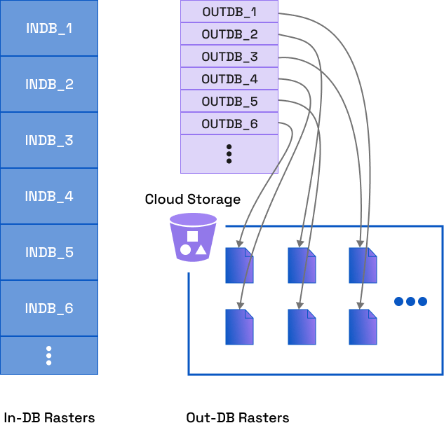 In WherobotsDB, we recommend Out-DB raster for your raster data, as it is more efficient and scalable. In this tutorial, we will show you how to create an Out-DB raster table and an In-DB raster table.
## Create an Out-DB Raster type column
Out-DB Rasters has the same data type with In-DB Rasters, they are all represented as `raster` primitive type in Havasu and can be loaded as `RasterUDT` objects in Sedona. If user has a table containing a `raster` column, it can have both In-DB and Out-DB rasters
in that column.
### Use the raster data loader
We can use the `raster` loader to load the data. The `raster` loader will load the binary files as out-db rasters and automatically split the raster into smaller tiles.
```scala theme={"system"}
var rawDf = sedona.read.format("raster").load("s3://wherobots-examples/data/eurosat_small/AnnualCrop/*.tif")
rawDf.createOrReplaceTempView("rawdf")
rawDf.show()
```
```java theme={"system"}
Dataset
In WherobotsDB, we recommend Out-DB raster for your raster data, as it is more efficient and scalable. In this tutorial, we will show you how to create an Out-DB raster table and an In-DB raster table.
## Create an Out-DB Raster type column
Out-DB Rasters has the same data type with In-DB Rasters, they are all represented as `raster` primitive type in Havasu and can be loaded as `RasterUDT` objects in Sedona. If user has a table containing a `raster` column, it can have both In-DB and Out-DB rasters
in that column.
### Use the raster data loader
We can use the `raster` loader to load the data. The `raster` loader will load the binary files as out-db rasters and automatically split the raster into smaller tiles.
```scala theme={"system"}
var rawDf = sedona.read.format("raster").load("s3://wherobots-examples/data/eurosat_small/AnnualCrop/*.tif")
rawDf.createOrReplaceTempView("rawdf")
rawDf.show()
```
```java theme={"system"}
Dataset rawDf = sedona.read().format("raster").load("s3://wherobots-examples/data/eurosat_small/AnnualCrop/*.tif")
rawDf.createOrReplaceTempView("rawdf")
rawDf.show()
```
```python theme={"system"}
rawDf = sedona.read.format("raster").load("s3://wherobots-examples/data/eurosat_small/AnnualCrop/*.tif")
rawDf.createOrReplaceTempView("rawdf")
rawDf.show()
```
The output will look like the following. We can see that the files are loaded as out-db rasters and divided into smaller tiles with the tile coordinates `x` and `y` attached to each tile.
```
+--------------------+---+---+
| rast| x| y|
+--------------------+---+---+
|OutDbGridCoverage...| 0| 0|
|OutDbGridCoverage...| 1| 0|
|OutDbGridCoverage...| 2| 0|
...
```
For more details about the `raster` loader, please refer to [Loading raster using the raster loader](/reference/wherobots-db/raster-data/raster-loader/#loading-raster-using-the-raster-loader).
### Use RS\_FromPath to create Out-DB Raster
User can create an out-db raster using [`RS_FromPath`](/reference/wherobots-db/raster-data/raster-loader/#rs_frompath) function:
```python theme={"system"}
df = sedona.sql("SELECT RS_FromPath('s3://wherobots-examples/data/eurosat_small/AnnualCrop/AnnualCrop_10.tif') as rast")
```
```scala theme={"system"}
val df = sedona.sql("SELECT RS_FromPath('s3://wherobots-examples/data/eurosat_small/AnnualCrop/AnnualCrop_10.tif') as rast")
```
```java theme={"system"}
Dataset df = sedona.sql("SELECT RS_FromPath('s3://wherobots-examples/data/eurosat_small/AnnualCrop/AnnualCrop_10.tif') as rast");
```
WherobotsDB allows adding multiple out-db rasters to one object. This example ensures the out-db raster will retrieve the raster only when required for computation:
```python theme={"system"}
df = sedona.read.format("binaryFile")
.option("recursiveFileLookup", "true").option("pathGlobFilter", "*.tif*")
.load("s3://wherobots-examples/data/eurosat_small/AnnualCrop/*.tif")
.drop("content").withColumn("rast", expr("RS_FromPath(path)"))
```
```scala theme={"system"}
val df = sedona.read.format("binaryFile")
.option("recursiveFileLookup", "true").option("pathGlobFilter", "*.tif*")
.load("s3://wherobots-examples/data/eurosat_small/AnnualCrop/*.tif")
.drop("content").withColumn("rast", expr("RS_FromPath(path)"))
```
```java theme={"system"}
Dataset df = sedona.read.format("binaryFile")
.option("recursiveFileLookup", "true").option("pathGlobFilter", "*.tif*")
.load("s3://wherobots-examples/data/eurosat_small/AnnualCrop/*.tif")
.drop("content").withColumn("rast", expr("RS_FromPath(path)"))
```
The result of `RS_FromPath` is an Out-db raster object, which can be stored in a raster column in a Havasu table.
### Retrieve the path of Out-DB Rasters
The rasters path of out-db rasters can be retrieved using [`RS_BandPath`](/reference/wherobots-db/raster-data/raster-loader/#rs_bandpath) function. It will give the path of the raster file in remote storage. If the argument is an in-db raster, `RS_BandPath` will return `NULL`.
```python theme={"system"}
df.selectExpr("RS_BandPath(rast)").show()
```
```scala theme={"system"}
df.selectExpr("RS_BandPath(rast)").show()
```
```java theme={"system"}
df.selectExpr("RS_BandPath(rast)").show();
```
```
+--------------------+
| rs_bandpath(rast)|
+--------------------+
|s3://wherobots-e...|
+--------------------+
```
### Divide and explode Out-DB Rasters
Large Out-DB rasters can be subdivided into tiles using `RS_TileExplode` function:
```python theme={"system"}
df.selectExpr("RS_TileExplode(rast) as (x, y, rast)").show()
```
```scala theme={"system"}
df.selectExpr("RS_TileExplode(rast) as (x, y, rast)").show()
```
```java theme={"system"}
df.selectExpr("RS_TileExplode(rast) as (x, y, rast)").show();
```
The rasters `RS_TileExplode` produces are also Out-DB rasters as long as the input raster is an Out-DB raster. These tiles reference different parts of the same raster file in remote storage, so they are very cheap to create.
```python theme={"system"}
df.selectExpr("RS_TileExplode(rast, 32, 32) as (x, y, rast)").show()
```
```scala theme={"system"}
df.selectExpr("RS_TileExplode(rast, 32, 32) as (x, y, rast)").show()
```
```java theme={"system"}
df.selectExpr("RS_TileExplode(rast, 32, 32) as (x, y, rast)").show();
```
```
+---+---+--------------------+
| x| y| rast|
+---+---+--------------------+
| 0| 0|OutDbGridCoverage...|
| 1| 0|OutDbGridCoverage...|
| 0| 1|OutDbGridCoverage...|
| 1| 1|OutDbGridCoverage...|
+---+---+--------------------+
```
### Create Out-DB Raster from STAC GeoJSON files
This method is useful when dealing with large raster datasets stored in external storage systems like Amazon S3, as it allows the Havasu table to store only the path to the raster file along with geo-referencing metadata.
The following examples shows how to read a STAC file using the GeoJSON reader, load raster data from the STAC file and write it as an out-db raster to a Havasu table.
```python theme={"system"}
# Read STAC file using GeoJSON reader
df = sedona.read.format("geojson").load("stac-file-path")
# Read GeoTIFF files as out-db rasters using RS_FromPath
df_rast = df.withColumn("rast", expr("RS_FromPath(assets.analytic.href)"))
# Writing the data into Havasu table
df_rast.writeTo("org_catalog.test_db.test_table").append()
```
```scala theme={"system"}
// Read STAC file using GeoJSON reader
val df = sedona.read.format("geojson").load("stac-file-path")
// Read GeoTIFF files as out-db rasters using RS_FromPath
val df_rast = df.withColumn("rast", expr("RS_FromPath(assets.analytic.href)"))
// Write the out-db raster data into a Havasu table
df_rast.writeTo("org_catalog.test_db.test_table").append()
```
```java theme={"system"}
// Read STAC file using GeoJSON reader
Dataset df = sedona.read.format("geojson").load("stac-file-path");
// Read GeoTIFF files as out-db rasters using RS_FromPath
Dataset df_rast = df.withColumn("rast", expr("RS_FromPath(assets.analytic.href)"));
// Write the out-db raster data into a Havasu table
df_rast.selectExpr("rast", "path AS data").writeTo("org_catalog.test_db.test_table").append();
```
### Supported Out-DB Storages
Havasu supports any storages that Hadoop supports, as long as the storage has an implementation of `org.apache.hadoop.fs.FileSystem` on the classpath of the Wherobots Cloud. In the above examples, we accessed out-db rasters stored on S3 using the S3A file system provided by Hadoop AWS. Following is a list of storages that are tested on Wherobots Cloud:
| Storage | Scheme | File System Class |
| ------- | --------- | ---------------------------------------- |
| Local | `file://` | `org.apache.hadoop.fs.LocalFileSystem` |
| S3 | `s3://` | `org.apache.hadoop.fs.s3a.S3AFileSystem` |
## Create an In-DB Raster type column
All raster operations in Spatial SQL require Raster type objects. Therefore, this should be the next step after loading the data.
### Load binary raster data
Assume we have a single raster data file called rasterData.tiff, [at Path](https://github.com/apache/sedona/blob/0eae42576c2588fe278f75cef3b17fee600eac90/spark/common/src/test/resources/raster/raster_with_no_data/test5.tiff).
Use the following code to load the data and create a WherobotsDB Dataframe.
```scala theme={"system"}
var rawDf = sedona.read.format("binaryFile").load(path_to_raster_data)
rawDf.createOrReplaceTempView("rawdf")
rawDf.show()
```
```java theme={"system"}
Dataset rawDf = sedona.read.format("binaryFile").load(path_to_raster_data)
rawDf.createOrReplaceTempView("rawdf")
rawDf.show()
```
```python theme={"system"}
rawDf = sedona.read.format("binaryFile").load(path_to_raster_data)
rawDf.createOrReplaceTempView("rawdf")
rawDf.show()
```
The output will look like this:
```
| path| modificationTime|length| content|
+--------------------+--------------------+------+--------------------+
|file:/Download/ra...|2023-09-06 16:24:...|174803|[49 49 2A 00 08 0...|
```
For multiple raster data files use the following code to load the data [from path](https://github.com/apache/sedona/blob/0eae42576c2588fe278f75cef3b17fee600eac90/spark/common/src/test/resources/raster/) and create raw DataFrame.
The above code works too for loading multiple raster data files. if the raster files are in separate directories and the option also makes sure that only `.tif` or `.tiff` files are being loaded.
```scala theme={"system"}
var rawDf = sedona.read.format("binaryFile").option("recursiveFileLookup", "true").option("pathGlobFilter", "*.tif*").load(path_to_raster_data_folder)
rawDf.createOrReplaceTempView("rawdf")
rawDf.show()
```
```java theme={"system"}
Dataset rawDf = sedona.read.format("binaryFile").option("recursiveFileLookup", "true").option("pathGlobFilter", "*.tif*").load(path_to_raster_data_folder);
rawDf.createOrReplaceTempView("rawdf");
rawDf.show();
```
```python theme={"system"}
rawDf = sedona.read.format("binaryFile").option("recursiveFileLookup", "true").option("pathGlobFilter", "*.tif*").load(path_to_raster_data_folder)
rawDf.createOrReplaceTempView("rawdf")
rawDf.show()
```
The output will look like this:
```
| path| modificationTime|length| content|
+--------------------+--------------------+------+--------------------+
|file:/Download/ra...|2023-09-06 16:24:...|209199|[4D 4D 00 2A 00 0...|
|file:/Download/ra...|2023-09-06 16:24:...|174803|[49 49 2A 00 08 0...|
|file:/Download/ra...|2023-09-06 16:24:...|174803|[49 49 2A 00 08 0...|
|file:/Download/ra...|2023-09-06 16:24:...| 6619|[49 49 2A 00 08 0...|
```
The content column in the raster table is still in the raw form, binary form.
Recursive file lookup will also work similarly for raster datasets in .asc file formats.
### From Geotiff
```sql theme={"system"}
SELECT RS_FromGeoTiff(content) AS rast, modificationTime, length, path FROM rawdf
```
To verify this, use the following code to print the schema of the DataFrame:
```sql theme={"system"}
rasterDf.printSchema()
```
The output will be like this:
```
root
|-- rast: raster (nullable = true)
|-- modificationTime: timestamp (nullable = true)
|-- length: long (nullable = true)
|-- path: string (nullable = true)
```
### From Arc Grid
The raster data is loaded the same way as `tiff` file, but the raster data is stored with the extension `.asc`, ASCII format. The following code creates a Raster type objects from binary data:
```sql theme={"system"}
SELECT RS_FromArcInfoAsciiGrid(content) AS rast, modificationTime, length, path FROM rawdf
```
## Raster's metadata
WherobotsDB has a function to get the metadata for the raster, and also a function to get the world file of the raster.
### Metadata
This function will return an array of metadata, it will have all the necessary information about the raster, Please refer to [RS\_MetaData](/reference/wherobots-db/raster-data/operators/RS_MetaData).
```sql theme={"system"}
SELECT RS_MetaData(rast) FROM rasterDf
```
Output for the following function will be:
```
[-1.3095817809482181E7, 4021262.7487925636, 512.0, 517.0, 72.32861272132695, -72.32861272132695, 0.0, 0.0, 3857.0, 1.0]
```
The first two elements of the array represent the real-world geographic coordinates (like longitude/latitude) of the raster image's top left pixel, while the next two elements represent the pixel dimensions of the raster.
### World File
There are two kinds of georeferences, GDAL and ESRI seen in [world files](https://en.wikipedia.org/wiki/World_file). For more information please refer to [RS\_GeoReference](/reference/wherobots-db/raster-data/accessors/RS_GeoReference).
```sql theme={"system"}
SELECT RS_GeoReference(rast, "ESRI") FROM rasterDf
```
The Output will be as follows:
```
72.328613
0.000000
0.000000
-72.328613
-13095781.645176
4021226.584486
```
World files are used to georeference and geolocate images by establishing an image-to-world coordinate transformation that assigns real-world geographic coordinates to the pixels of the image.