> ## Documentation Index
> Fetch the complete documentation index at: https://docs.wherobots.com/llms.txt
> Use this file to discover all available pages before exploring further.

# Matching GPS traces to road networks

> Learn how to use Wherobots Matcher to align GPS traces with road networks, improving the accuracy of navigation and location-based services.

## Introduction to Map Matching with Matcher

In GPS-based navigation systems, devices often provide GPS coordinates that might be imprecise and don't necessarily
align with actual road networks. This discrepancy can be addressed by a process known as map matching, which aligns
these potentially inaccurate GPS points to their correct road segments, ensuring the accuracy of navigation routes and
providing a seamless navigation experience for users.

## Import Matcher Functions

To leverage the map matching functionalities offered by Wherobots Matcher, you need to import the relevant class. The
MapMatching class from the matcher module provides these capabilities:

<Tabs>
  <Tab title="Python">
    ```python theme={"system"}
    from wherobots import matcher
    ```
  </Tab>

  <Tab title="Scala">
    ```scala theme={"system"}
    import com.wherobots.Matcher
    ```
  </Tab>

  <Tab title="Java">
    ```java theme={"system"}
    import com.wherobots.Matcher;
    ```
  </Tab>
</Tabs>

## Loading OSM Data

Once you've accessed the MapMatching class, the next step is to load data from the OpenStreetMap (OSM). Wherobots Matcher
supports loading an OSM file into a Sedona DataFrame. This DataFrame is then enriched with the necessary attributes for
map matching.

If your OSM data is saved at a local path like data/osm.xml, or on a remote storage such as an AWS S3 path, you can load
this data using the following code:

<Tabs>
  <Tab title="Python">
    ```python theme={"system"}
    dfEdge = matcher.load_osm("data/osm.xml", "[car]")
    dfEdge.show(5)
    ```
  </Tab>

  <Tab title="Scala">
    ```scala theme={"system"}
    val dfEdge = Matcher.loadOSM(resourceFolder + "osm2.xml", "[car]")
    dfEdge.show(5)
    ```
  </Tab>

  <Tab title="Java">
    ```java theme={"system"}
    Dataset dfEdge = Matcher.loadOSM(resourceFoler + "data/osm2.xml", "[car]");
    dfEdge.show(5);
    ```
  </Tab>
</Tabs>

The `[car]` parameter is the road type filter, which can be used to filter out road segments that are not suitable for
cars.

Upon executing the above code, you can expect an output that aligns with the example below:

```
+--------------------+----------+--------+----------+-----------+----------+-----------+
|            geometry|       src|     dst|   src_lat|    src_lon|   dst_lat|    dst_lon|
+--------------------+----------+--------+----------+-----------+----------+-----------+
|LINESTRING (-83.0...|  62545092|62545090| 42.350883| -83.071323|42.3502907|-83.0711018|
|LINESTRING (-83.0...|7592807480|62545090|42.3495189|-83.0708043|42.3502907|-83.0711018|
|LINESTRING (-83.0...|8129132226|62545316| 42.363371|-83.0546103|42.3634571|-83.0546522|
|LINESTRING (-83.0...|  62859327|62545316| 42.363539| -83.054686|42.3634571|-83.0546522|
|LINESTRING (-83.0...|8129132225|62545316|42.3635311|-83.0547655|42.3634571|-83.0546522|
+--------------------+----------+--------+----------+-----------+----------+-----------+
only showing top 5 rows
```

This table represents the top five rows of the loaded OSM data, showcasing the geometry and attributes of the road
segments.

In the context of the table:

* `src` (source): Represents the starting point or origin of a path. Each src has associated coordinates given by
  src\_lat and src\_lon.
* `dst` (destination): Refers to the endpoint of a path. Each dst has coordinates represented by dst\_lat and
  dst\_lon.

Simply put, the table illustrates various paths in a network, detailing their starting (src) and ending (dst) points
with corresponding geographic coordinates.

## Create Sedona DataFrame of GPS Trips

With the Sedona library, which provides APIs and data structures for spatial operations, you can transform a list of GPS
tracks into a Sedona DataFrame where each track is represented as a LineString.

Follow these steps to create a Sedona DataFrame of GPS trips:

1. Format the given GPS coordinates into strings that can be converted into LineString objects.
2. Next, Use Sedona's API to create a DataFrame of these LineString objects.

Here are the GPS tracks,

<Tabs>
  <Tab title="Python">
    ```python theme={"system"}
    gps_tracks = [
        (42.355618, -83.054237), (42.35562, -83.054238), (42.355615, -83.054253), (42.355684, -83.054297), (42.355719, -83.054198),
        (42.355781, -83.054022), (42.355749, -83.054001), (42.355781, -83.054022), (42.355719, -83.054198), (42.35565, -83.054155),
        (42.355587, -83.054116), (42.355656, -83.053914), (42.35573, -83.053715), (42.355749, -83.053728), (42.35573, -83.053715),
        (42.355656, -83.053914), (42.355722, -83.05396), (42.355839, -83.053635), (42.355918, -83.053637), (42.355993, -83.053428),
        (42.355967, -83.053411), (42.355993, -83.053428), (42.355918, -83.053637), (42.355839, -83.053635), (42.355886, -83.053504),
        (42.355999, -83.053194), (42.356038, -83.053086), (42.356027, -83.053079), (42.356038, -83.053086), (42.356105, -83.052904),
        (42.356126, -83.052918), (42.356105, -83.052904), (42.355999, -83.053194), (42.355933, -83.053149), (42.35602, -83.052916),
        (42.35609, -83.052727), (42.356102, -83.052735), (42.35609, -83.052727), (42.35602, -83.052916), (42.355933, -83.053149),
        (42.355999, -83.053194), (42.356243, -83.052523), (42.356265, -83.052537), (42.356243, -83.052523), (42.3563, -83.052367),
        (42.356273, -83.052349), (42.3563, -83.052367), (42.356362, -83.052196), (42.356388, -83.052125), (42.356409, -83.052139),
        (42.356407, -83.052145), (42.356409, -83.052139), (42.35646, -83.052173), (42.356499, -83.052073), (42.356424, -83.052024),
        (42.356348, -83.051973), (42.35638, -83.051886), (42.356395, -83.051847), (42.356423, -83.051866), (42.356395, -83.051847),
        (42.35638, -83.051886), (42.356348, -83.051973), (42.356424, -83.052024), (42.356457, -83.051932), (42.356562, -83.051641),
        (42.356578, -83.051652), (42.356562, -83.051641), (42.35672, -83.051204), (42.356732, -83.051212), (42.35672, -83.051204),
        (42.356722, -83.051198), (42.356795, -83.050995), (42.356827, -83.051015), (42.356816, -83.051046), (42.356827, -83.051015),
        (42.356795, -83.050995), (42.356724, -83.050952), (42.356761, -83.050841), (42.356838, -83.050876), (42.356865, -83.050894),
        (42.356859, -83.050911), (42.356865, -83.050894), (42.356838, -83.050876), (42.356923, -83.050643), (42.356891, -83.050622),
        (42.356923, -83.050643), (42.356999, -83.050433), (42.356927, -83.050386), (42.356953, -83.050315), (42.356978, -83.050332),
        (42.356953, -83.050315), (42.356927, -83.050386), (42.35684, -83.050328), (42.356827, -83.050364), (42.35684, -83.050328),
        (42.356722, -83.050249), (42.35674, -83.050198), (42.356722, -83.050249), (42.356506, -83.050105), (42.356494, -83.050139),
        (42.356506, -83.050105), (42.356443, -83.050063), (42.356431, -83.050096), (42.356443, -83.050063), (42.356388, -83.050025),
        (42.356399, -83.049994), (42.356388, -83.050025), (42.356357, -83.050005), (42.356345, -83.049897), (42.356349, -83.049884),
        (42.35638, -83.049903), (42.356349, -83.049884), (42.356386, -83.049777), (42.356407, -83.04979), (42.356386, -83.049777),
        (42.356464, -83.049549), (42.356459, -83.049533)
    ]
    ```
  </Tab>

  <Tab title="Scala">
    ```scala theme={"system"}
    val gps_tracks: List[(Double, Double)] = List(
      (42.355618, -83.054237), (42.35562, -83.054238), (42.355615, -83.054253), (42.355684, -83.054297), (42.355719, -83.054198),
      (42.355781, -83.054022), (42.355749, -83.054001), (42.355781, -83.054022), (42.355719, -83.054198), (42.35565, -83.054155),
      (42.355587, -83.054116), (42.355656, -83.053914), (42.35573, -83.053715), (42.355749, -83.053728), (42.35573, -83.053715),
      (42.355656, -83.053914), (42.355722, -83.05396), (42.355839, -83.053635), (42.355918, -83.053637), (42.355993, -83.053428),
      (42.355967, -83.053411), (42.355993, -83.053428), (42.355918, -83.053637), (42.355839, -83.053635), (42.355886, -83.053504),
      (42.355999, -83.053194), (42.356038, -83.053086), (42.356027, -83.053079), (42.356038, -83.053086), (42.356105, -83.052904),
      (42.356126, -83.052918), (42.356105, -83.052904), (42.355999, -83.053194), (42.355933, -83.053149), (42.35602, -83.052916),
      (42.35609, -83.052727), (42.356102, -83.052735), (42.35609, -83.052727), (42.35602, -83.052916), (42.355933, -83.053149),
      (42.355999, -83.053194), (42.356243, -83.052523), (42.356265, -83.052537), (42.356243, -83.052523), (42.3563, -83.052367),
      (42.356273, -83.052349), (42.3563, -83.052367), (42.356362, -83.052196), (42.356388, -83.052125), (42.356409, -83.052139),
      (42.356407, -83.052145), (42.356409, -83.052139), (42.35646, -83.052173), (42.356499, -83.052073), (42.356424, -83.052024),
      (42.356348, -83.051973), (42.35638, -83.051886), (42.356395, -83.051847), (42.356423, -83.051866), (42.356395, -83.051847),
      (42.35638, -83.051886), (42.356348, -83.051973), (42.356424, -83.052024), (42.356457, -83.051932), (42.356562, -83.051641),
      (42.356578, -83.051652), (42.356562, -83.051641), (42.35672, -83.051204), (42.356732, -83.051212), (42.35672, -83.051204),
      (42.356722, -83.051198), (42.356795, -83.050995), (42.356827, -83.051015), (42.356816, -83.051046), (42.356827, -83.051015),
      (42.356795, -83.050995), (42.356724, -83.050952), (42.356761, -83.050841), (42.356838, -83.050876), (42.356865, -83.050894),
      (42.356859, -83.050911), (42.356865, -83.050894), (42.356838, -83.050876), (42.356923, -83.050643), (42.356891, -83.050622),
      (42.356923, -83.050643), (42.356999, -83.050433), (42.356927, -83.050386), (42.356953, -83.050315), (42.356978, -83.050332),
      (42.356953, -83.050315), (42.356927, -83.050386), (42.35684, -83.050328), (42.356827, -83.050364), (42.35684, -83.050328),
      (42.356722, -83.050249), (42.35674, -83.050198), (42.356722, -83.050249), (42.356506, -83.050105), (42.356494, -83.050139),
      (42.356506, -83.050105), (42.356443, -83.050063), (42.356431, -83.050096), (42.356443, -83.050063), (42.356388, -83.050025),
      (42.356399, -83.049994), (42.356388, -83.050025), (42.356357, -83.050005), (42.356345, -83.049897), (42.356349, -83.049884),
      (42.35638, -83.049903), (42.356349, -83.049884), (42.356386, -83.049777), (42.356407, -83.04979), (42.356386, -83.049777),
      (42.356464, -83.049549), (42.356459, -83.049533)
    )
    ```
  </Tab>

  <Tab title="Java">
    ```java theme={"system"}
    double[][] gps_tracks = {
        {42.355618, -83.054237}, {42.35562, -83.054238}, {42.355615, -83.054253}, {42.355684, -83.054297}, {42.355719, -83.054198},
        {42.355781, -83.054022}, {42.355749, -83.054001}, {42.355781, -83.054022}, {42.355719, -83.054198}, {42.35565, -83.054155},
        {42.355587, -83.054116}, {42.355656, -83.053914}, {42.35573, -83.053715}, {42.355749, -83.053728}, {42.35573, -83.053715},
        {42.355656, -83.053914}, {42.355722, -83.05396}, {42.355839, -83.053635}, {42.355918, -83.053637}, {42.355993, -83.053428},
        {42.355967, -83.053411}, {42.355993, -83.053428}, {42.355918, -83.053637}, {42.355839, -83.053635}, {42.355886, -83.053504},
        {42.355999, -83.053194}, {42.356038, -83.053086}, {42.356027, -83.053079}, {42.356038, -83.053086}, {42.356105, -83.052904},
        {42.356126, -83.052918}, {42.356105, -83.052904}, {42.355999, -83.053194}, {42.355933, -83.053149}, {42.35602, -83.052916},
        {42.35609, -83.052727}, {42.356102, -83.052735}, {42.35609, -83.052727}, {42.35602, -83.052916}, {42.355933, -83.053149},
        {42.355999, -83.053194}, {42.356243, -83.052523}, {42.356265, -83.052537}, {42.356243, -83.052523}, {42.3563, -83.052367},
        {42.356273, -83.052349}, {42.3563, -83.052367}, {42.356362, -83.052196}, {42.356388, -83.052125}, {42.356409, -83.052139},
        {42.356407, -83.052145}, {42.356409, -83.052139}, {42.35646, -83.052173}, {42.356499, -83.052073}, {42.356424, -83.052024},
        {42.356348, -83.051973}, {42.35638, -83.051886}, {42.356395, -83.051847}, {42.356423, -83.051866}, {42.356395, -83.051847},
        {42.35638, -83.051886}, {42.356348, -83.051973}, {42.356424, -83.052024}, {42.356457, -83.051932}, {42.356562, -83.051641},
        {42.356578, -83.051652}, {42.356562, -83.051641}, {42.35672, -83.051204}, {42.356732, -83.051212}, {42.35672, -83.051204},
        {42.356722, -83.051198}, {42.356795, -83.050995}, {42.356827, -83.051015}, {42.356816, -83.051046}, {42.356827, -83.051015},
        {42.356795, -83.050995}, {42.356724, -83.050952}, {42.356761, -83.050841}, {42.356838, -83.050876}, {42.356865, -83.050894},
        {42.356859, -83.050911}, {42.356865, -83.050894}, {42.356838, -83.050876}, {42.356923, -83.050643}, {42.356891, -83.050622},
        {42.356923, -83.050643}, {42.356999, -83.050433}, {42.356927, -83.050386}, {42.356953, -83.050315}, {42.356978, -83.050332},
        {42.356953, -83.050315}, {42.356927, -83.050386}, {42.35684, -83.050328}, {42.356827, -83.050364}, {42.35684, -83.050328},
        {42.356722, -83.050249}, {42.35674, -83.050198}, {42.356722, -83.050249}, {42.356506, -83.050105}, {42.356494, -83.050139},
        {42.356506, -83.050105}, {42.356443, -83.050063}, {42.356431, -83.050096}, {42.356443, -83.050063}, {42.356388, -83.050025},
        {42.356399, -83.049994}, {42.356388, -83.050025}, {42.356357, -83.050005}, {42.356345, -83.049897}, {42.356349, -83.049884},
        {42.35638, -83.049903}, {42.356349, -83.049884}, {42.356386, -83.049777}, {42.356407, -83.04979}, {42.356386, -83.049777},
        {42.356464, -83.049549}, {42.356459, -83.049533}
    };
    ```
  </Tab>
</Tabs>

Use the following code to create the Sedona DataFrame of LineStrings/GPS paths:

<Tabs>
  <Tab title="Python">
    ```python theme={"system"}
    ids = []
    lines = []
    i = j = k = 0
    lineStr = ""

    while k < len(gps_tracks):
      if j == 15 or k == len(gps_tracks)-1:
        ids.append(i)
        lines.append(lineStr)
        i += 1
        j = 0
        lineStr = ""
      if j == 0:
        lineStr += str(gps_tracks[j][1]) + "," + str(gps_tracks[j][0])
      else:
        lineStr += "," + str(gps_tracks[j][1]) + "," + str(gps_tracks[j][0])
      j += 1
      k += 1

    df_paths = sedona.createDataFrame(zip(ids, lines), ["ids", "lon_lat_seq"])
    df_paths = df_paths.withColumn("geometry", expr("ST_LineStringFromText(lon_lat_seq, ',')")).drop("lon_lat_seq");
    df_paths.show(5);
    ```
  </Tab>

  <Tab title="Scala">
    ```scala theme={"system"}
    var ids = List[Int]()
    var lines = List[String]()
    var i = 0
    var j = 0
    var k = 0
    var lineStr = ""

    while (k < gps_tracks.length) {
      if (j == 15 || k == gps_tracks.length - 1) {
        ids = ids :+ i
        lines = lines :+ lineStr
        i += 1
        j = 0
        lineStr = ""
      }
      if (j == 0) {
        lineStr += gps_tracks(j)._2 + "," + gps_tracks(j)._1
      } else {
        lineStr += "," + gps_tracks(j)._2 + "," + gps_tracks(j)._1
      }
      j += 1
      k += 1
    }

    val dfPaths = ids.zip(lines).toDF("ids", "lon_lat_seq")
    .withColumn("geometry", expr("ST_LineStringFromText(lon_lat_seq, ',')"))
    .drop("lon_lat_seq")

    dfPaths.show(5)
    ```
  </Tab>

  <Tab title="Java">
    ```java theme={"system"}
    List<Integer> ids = new ArrayList<>();
    List<String> lines = new ArrayList<>();
    int i = 0;
    int j = 0;
    int k = 0;
    String lineStr = "";

    while (k < gps_tracks.length) {
      if (j == 15 || k == gps_tracks.length - 1) {
        ids.add(i);
        lines.add(lineStr);
        i += 1;
        j = 0;
        lineStr = "";
      }
      if (j == 0) {
        lineStr += gps_tracks[j][1] + "," + gps_tracks[j][0];
      } else {
        lineStr += "," + gps_tracks[j][1] + "," + gps_tracks[j][0];
      }
      j += 1;
      k += 1;
    }

    Dataset<Row> dfPaths = org.apache.spark.sql.functions.zip(ids, lines).toDF("ids", "lon_lat_seq")
        .withColumn("geometry", functions.expr("ST_LineStringFromText(lon_lat_seq, ',')"))
        .drop("lon_lat_seq");

    dfPaths.show(5);
    ```
  </Tab>
</Tabs>

Output will be similar to the following:

```
+---+--------------------+
|ids|            geometry|
+---+--------------------+
|  0|LINESTRING (-83.0...|
|  1|LINESTRING (-83.0...|
|  2|LINESTRING (-83.0...|
|  3|LINESTRING (-83.0...|
|  4|LINESTRING (-83.0...|
+---+--------------------+
only showing top 5 rows
```

## Map Matching on Batch Data

Now that you have both the OSM edges DataFrame and the GPS trips DataFrame, you're ready to perform map matching. The
below code is used to execute map matching and display the top 5 rows of the resulting DataFrame.

<Tabs>
  <Tab title="Python">
    ```python theme={"system"}
    result_df = matcher.match(df_edge, df_paths, "geometry", "geometry")
    result_df.show(5)
    ```
  </Tab>

  <Tab title="Scala">
    ```scala theme={"system"}
    val resultDf = Matcher.match(dfEdge, dfPaths, "geometry", "geometry")
    resultDf.show(5)
    ```
  </Tab>

  <Tab title="Java">
    ```java theme={"system"}
    Dataset matchingResultDf = Matcher.match(edgesDf, pathsSpatialDf, "geometry", "geometry");
    matchingResultDf.show();
    ```
  </Tab>
</Tabs>

The parameters in the method `match` are as follows:

* dfEdge: A DataFrame of road segments from OpenStreetMap.
* dfPaths: A DataFrame of GPS paths to be aligned to roads.
* colEdgesGeom: The column in dfEdge holding road geometry.
* colPathsGeom: The column in dfPaths holding GPS path geometry.
* idFieldName: Optional - The column in dfPaths DataFrame that contains the unique identifier for each GPS trip. if not
  provided, the first non-geometry column is used.

The output should be similar to the following table:

```
+---+--------------------+--------------------+--------------------+
|ids|     observed_points|      matched_points|       matched_nodes|
+---+--------------------+--------------------+--------------------+
|  4|[[-83.054237, 42....|[[-83.05423815457...|[4071942207, 6260...|
|  7|[[-83.054237, 42....|[[-83.05423815457...|[4071942207, 6260...|
|  1|[[-83.054237, 42....|[[-83.05423815457...|[4071942207, 6260...|
|  3|[[-83.054237, 42....|[[-83.05423815457...|[4071942207, 6260...|
|  5|[[-83.054237, 42....|[[-83.05423815457...|[4071942207, 6260...|
+---+--------------------+--------------------+--------------------+
only showing top 5 rows
```

## Visualizing the result using SedonaKepler

To visualize the map matching result using SedonaKepler, you can use the following code:

```python theme={"system"}
my_map = SedonaKepler.create_map()
SedonaKepler.add_df(my_ap, dfEdge, name="Road Network")
SedonaKepler.add_df(my_ap, result_df.select("observed_points"), name="Observed Points")
SedonaKepler.add_df(my_ap, result_df.select("matched_points"), name="Matched Points")

my_map
```

Below is a visual representation of an example map matching result:

* Red Line: Illustrates the raw GPS trajectories, which capture the vehicle's original movement as recorded by the GPS
  device.
* Green Line: Highlights the trajectories after map matching, reflecting a refined path that aligns the GPS observations
  with the actual road network.

<Frame>
  <img src="https://mintcdn.com/wherobots/CqOVZhxtIAx4Gp_9/images/tutorials/wherobotsai/SedonaKepler_viz.png?fit=max&auto=format&n=CqOVZhxtIAx4Gp_9&q=85&s=f34505c5e5f6fd0d2195e22a88c4abd9" alt="SedonaKepler" width="1672" height="1532" data-path="images/tutorials/wherobotsai/SedonaKepler_viz.png" />
</Frame>

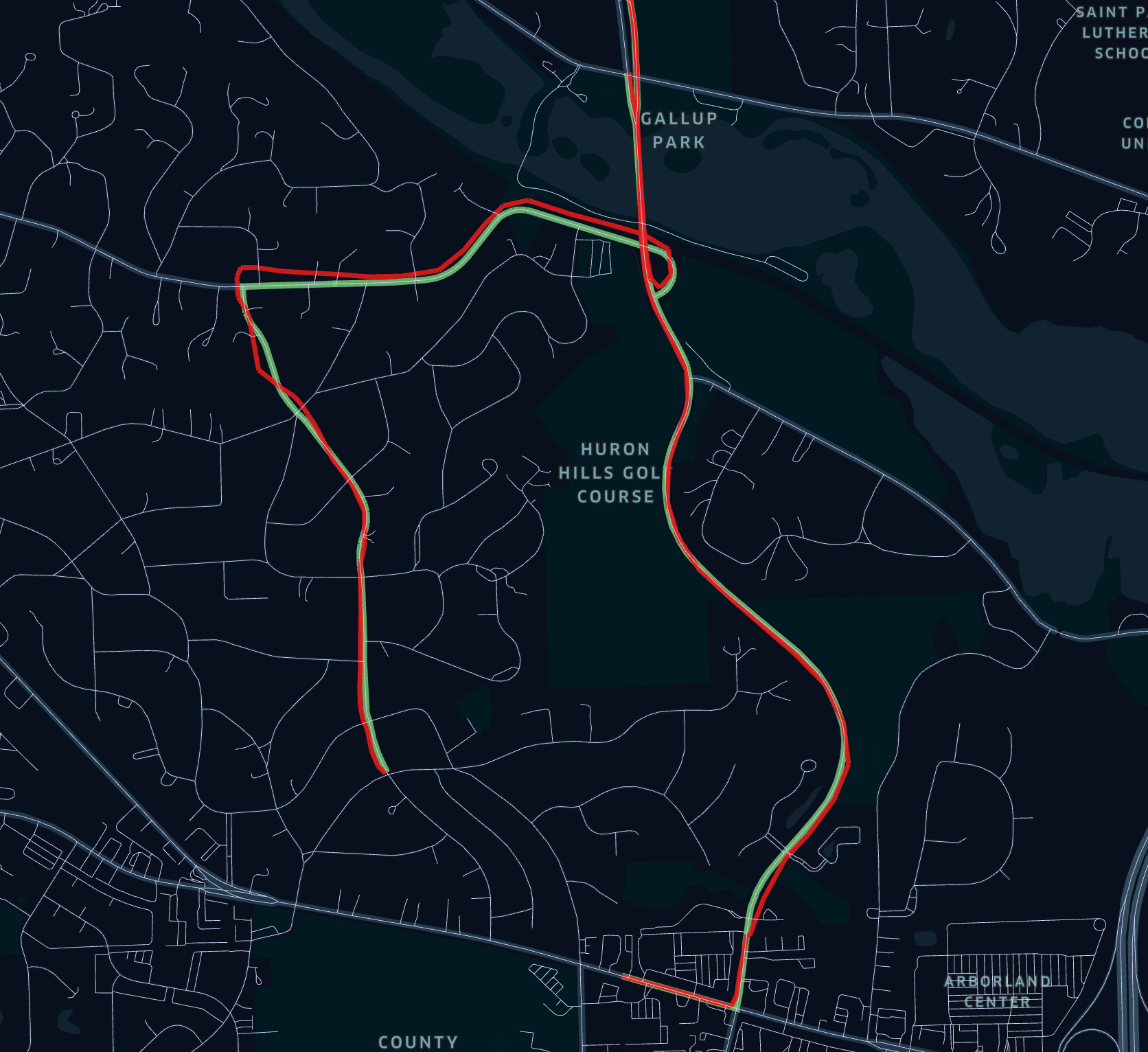A comparison of the red and green lines reveals the adjustments made by the map-matching algorithm, ensuring that raw
GPS data corresponds accurately with established roadways and provides a precise depiction of the vehicle's journey
through the network.

## Advanced Configuration

Wherobots map matching has several advanced configs that can be set through `Config`:

<Tabs>
  <Tab title="Python">
    ```python theme={"system"}
    config = SedonaContext.builder() .\
        config("wherobots.tools.mm.maxdist","50.0"). \
        getOrCreate()
    sedona = SedonaContext.create(config)
    ```
  </Tab>

  <Tab title="Scala">
    ```scala theme={"system"}
    val config = SedonaContext.builder().
        config("wherobots.tools.mm.maxdist","50.0").
        .getOrCreate()
    val sedona = SedonaContext.create(config)
    ```
  </Tab>

  <Tab title="Java">
    ```java theme={"system"}
    SparkSession config = SedonaContext.builder()
                .config("wherobots.tools.mm.maxdist","50.0")
                .appName("SparkSedonaExample")
                .getOrCreate();
    SparkSession sedona = SedonaContext.create(config);
    ```
  </Tab>
</Tabs>

These configurations can also be tuned when the SedonaContext was already created:

<Tabs>
  <Tab title="Python">
    ```python theme={"system"}
    sedona.conf.set("wherobots.tools.mm.maxdist", "50.0")
    ```
  </Tab>

  <Tab title="Scala">
    ```scala theme={"system"}
    sedona.conf.set("wherobots.tools.mm.maxdist", "50.0")
    ```
  </Tab>

  <Tab title="Java">
    ```java theme={"system"}
    sedona.conf().set("wherobots.tools.mm.maxdist", "50.0");
    ```
  </Tab>
</Tabs>

### Explanation

#### How Distributed Map-Matching Works

Wherobots runs batch map-matching on a large collection of trajectories in a distributed manner. The map-matching process is divided into two phases: *distributing workloads* and *local map-matching*. The *distributing workloads* phase rearranges the trajectories and the road segments near those trajectories to the same partition, and the *local map-matching* phase performs map-matching on each partition, where we already have trajectories and their surrounding road network co-located.

#### Parameters for Distributing Map-Matching Workloads

* wherobots.tools.mm.numspatialpartitions
  * Number of spatial partitions generated in the spatial join phase. This controls the parallelism of performing spatial join between trajectories and road networks. A recommended value is 10 \* number of executor cores.
    * Default value: None
    * Possible values: any positive integer value

#### The Local Map-Matching Algorithm

The local map-matching algorithm is based on a Hidden Markov Model (HMM), which is popularized by the paper [Hidden Markov Map Matching Through Noise and Sparseness](https://dl.acm.org/doi/10.1145/1653771.1653818). Wherobots implements a variation of this algorithm.

#### Parameters for the Local Map-Matching Algorithm

* wherobots.tools.mm.matcher
  * The algorithm for the local map matcher. The legacy mode works better for dense trajectories (high sampling rate) while the advanced mode works better for sparse trajectories (low sampling rate).
  * Default value: legacy
  * Possible values: legacy, advanced
* wherobots.tools.mm.adv.gpsaccuracy
  * The GPS accuracy of the input data, in the unit of meters. This controls the search radius of each observation. For sparse data, a higher value (e.g., 40 meters) will improve the accuracy but decrease the speed.
  * Default value: 20
  * Possible values: any positive integer value
* wherobots.tools.mm.adv.partialmatch
  * The local map matching algorithm will terminate early if it cannot find matches for every observation of a trip and the result will be a partial match of the original trip. This parameter controls if partial matches should be included in the output. If false, partial matches will become `LineString EMPTY` in the final output DataFrame.
  * Defalue value: false
  * Possible values: true, false